Competitive equilibrium with one-period Arrow securities
1. Competitive equilibrium with one-period Arrow securities
1.1. Summary
Following descriptions in section 9.3.3 of RMT5 chapter 9, we briefly recall the set up of a competitive equilibrium of a pure exchange economy with complete markets in one-period Arrow securities.
When endowments \(y^i(s)\) are all functions of a common Markov state \(s\), the pricing kernel takes the form \(Q(s'|s)\).
These enable us to provide a recursive formulation of the consumer’s optimization problem.
Consumer \(i\)’s state at time \(t\) is its financial wealth \(a^i_t\) and Markov state \(s_t\).
Let \(v^i(a,s)\) be the optimal value of consumer \(i\)’s problem starting from state \((a, s)\).
\(v^i(a,s)\) is the maximum expected discounted utility that consumer \(i\) with current financial wealth \(a\) can attain in state \(s\).
The value function satisfies the Bellman equation
where maximization is subject to the budget constraint
and also
with the second constraint evidently being a set of state-by-state debt limits.
Note that the value function and decision rule that solve the Bellman equation implicitly depend on the pricing kernel \(Q(\cdot \vert \cdot)\) because it appears in the agent’s budget constraint.
Use the first-order conditions for the problem on the right of the Bellman equation and a Benveniste-Scheinkman formula and rearrange to get
where it is understood that \(c_t^i = c^i(s_t)\) and \(c_{t+1}^i = c^i(s_{t+1})\).
A recursive competitive equilibrium is an initial distribution of wealth \(\vec a_0\), a set of borrowing limits \(\{\bar A^i(s)\}_{i=1}^I\), a pricing kernel \(Q(s' | s)\), sets of value functions \(\{v^i(a,s)\}_{i=1}^I\), and decision rules \(\{c^i(s), a^i(s)\}_{i=1}^I\) such that
The state-by-state borrowing constraints satisfy the recursion
For all \(i\), given \(a^i_0\), \(\bar A^i(s)\), and the pricing kernel, the value functions and decision rules solve the consumer’s problem;
For all realizations of \(\{s_t\}_{t=0}^\infty\), the consumption and asset portfolios \(\{\{c^i_t,\) \(\{\hat a^i_{t+1}(s')\}_{s'}\}_i\}_t\) satisfy \(\sum_i c^i_t = \sum_i y^i(s_t)\) and \(\sum_i \hat a_{t+1}^i(s') = 0\) for all \(t\) and \(s'\).
The initial financial wealth vector \(\vec a_0\) satisfies \(\sum_{i=1}^I a_0^i = 0 \).
The third condition asserts that there are zero net aggregate claims in all Markov states.
The fourth condition asserts that the economy is closed and starts off from a position in which there are zero net claims in the aggregate.
If an allocation and prices in a recursive competitive equilibrium are to be consistent with the equilibrium allocation and price system that prevail in a corresponding complete markets economy with all trades occurring at time \(0\), we must impose that \(a_0^i = 0\) for \(i = 1, \ldots , I\).
That is what assures that at time \(0\) the present value of each agent’s consumption equals the present value of his endowment stream, the single budget constraint in arrangement with all trades occurring at time \(0\).
Starting the system off with \(a_0^i =0 \ \forall i\) has a striking implication that we can call state variable degeneracy.
Thus, although there are two state variables in the value function \(v^i(a,s)\), within a recursive competitive equilibrium starting from \(a_0^i = 0 \ \forall i\) at the starting Markov state \(s_0\), two outcomes prevail:
\(a_0^i = 0 \) for all \(i\) whenever the Markov state \(s_t\) returns to \(s_0\).
Financial wealth \(a\) is an exact function of the Markov state \(s\).
The first finding asserts that each household recurrently visits the zero financial wealth state with which he began life.
The second finding asserts that the exogenous Markov state is all we require to track an individual.
Financial wealth turns out to be redundant.
This outcome depends critically on there being complete markets in Arrow securities.
1.2. Computing and Bellmanizing
This notebook is a laboratory for experimenting with instances of a pure exchange economy with
Markov endowments
Complete markets in one period Arrow state-contingent securities
Discounted expected utility preferences of a kind often specified in macro and finance
Common preferences across agents
Common beliefs across agents
A CRRA one-period utility function that implies the existence of a representative consumer whose consumption process can be plugged into a formula for the pricing kernel for one-step Arrow securities and thereby determine equilbrium prices before determing an equilibrium distribution of wealth
Diverse endowments across agents that provide motivations for reallocating goods across time and Markov states
We impose enough restrictions to allow us to Bellmanize competitive equilibrium prices and quantities
We can use Bellman equations to compute
asset prices
continuation wealths
state-by-state natural debt limits
As usual, we start with Python imports
import numpy as np
import matplotlib.pyplot as plt
%matplotlib inline
np.set_printoptions(suppress=True)
1.3. Markov asset prices primer
Let’s start with a brief summary of formulas for computing asset prices in a Markov setting.
The setup assumes the following infrastructure
Markov states: \(s \in S = \left[\bar{s}_1, \ldots, \bar{s}_n \right]\) governed by an \(n\)-state Markov chain with transition probability
A collection \(k=1,\ldots, K\) of \(n \times 1\) vectors of \(K\) assets that pay off \(d^k\left(s\right)\) in state \(s\)
An \(n \times n\) matrix pricing kernel \(Q\) for one-period Arrow securities, where \( Q_{ij}\) = price at time \(t\) in state \(s_t = \bar s_i\) of one unit of consumption when \(s_{t+1} = \bar s_j\) at time \(t+1\):
The price of risk-free one-period bond in state \(i\) is \(R_i^{-1} = \sum_{j}Q_{i,j}\)
The gross rate of return on a one-period risk-free bond Markov state \(\bar s_i\) is \(R_i = (\sum_j Q_{i,j})^{-1}\)
At this point, we’ll take the pricing kernel \(Q\) as exogenous, i.e., determined outside the model
Two examples would be
\( Q = \beta P \) where \(\beta \in (0,1) \)
\(Q = S P \) where \(S\) is an \(n \times n\) matrix of stochastic discount factors
We’ll write down implications of Markov asset pricing in a nutshell for two types of assets
the price in Markov state \(s\) at time \(t\) of a cum dividend stock that entitles the owner at the beginning of time \(t\) to the time \(t\) dividend and the option to sell the asset at time \(t+1\). The price evidently satisfies \(p^k(\bar s_i) = d^k(\bar s_i) + \sum_j Q_{ij} p^k(\bar s_j) \) which implies that the vector \(p^k\) satisfies \(p^k = d^k + Q p^k\) which implies the formula
the price in Markov state \(s\) at time \(t\) of an ex dividend stock that entitles the owner at the end of time \(t\) to the time \(t+1\) dividend and the option to sell the stock at time \(t+1\). The price is
Below, we describe an equilibrium model with trading of one-period Arrow securities in which the pricing kernel is endogenous.
In constructing our model, we’ll repeatedly encounter formulas that remind us of our asset pricing formulas.
1.4. Multi-step-forward transition probabilities and pricing kernels
The \((i,j)\) component of the \(k\)-step ahead transition probability \(P^k\) is
The \((i,j)\) component of the \(k\)-step ahead pricing kernel \(Q^k\) is
We’ll use these objects to state the following useful facts
1.5. Laws of iterated expectations and values
A law of iterated values has a mathematical structure that parallels the law of iterated expectations
We can describe its structure readily in the Markov setting of this lecture
Recall the following recursion satisfied \(j\) step ahead transition probabilites for our finite state Markov chain:
We can use this recursion to verify the law of iterated expectations applied to computing the conditional expectation of a random variable \(d(s_{t+j})\) conditioned on \(s_t\) via the following string of equalities
The pricing kernel for \(j\) step ahead Arrow securities satisfies the recursion
The time \(t\) value in Markov state \(s_t\) of a time \(t+j\) payout \(d(s_{t+j})\) is
The law of iterated values states
We verify it by pursuing the following a string of inequalities that are counterparts to those we used to verify the law of iterated expectations:
1.6. General equilibrium model (pure exchange)
1.6.1. Inputs
Markov states: \(s \in S = \left[\bar{s}_1, \ldots, \bar{s}_n \right]\) governed by an \(n\)-state Markov chain with transition probability
A collection of \(K \times 1\) vectors of individual \(k\) endowments: \(y^k\left(s\right), k=1,\ldots, K\)
An \(n \times 1\) vector of aggregate endowment: \(y\left(s\right) \equiv \sum_{k=1}^K y^k\left(s\right)\)
A collection of \(K \times 1\) vectors of individual \(k\) consumptions: \(c^k\left(s\right), k=1,\ldots, K\)
A collection of restrictions on feasible consumption allocations for \(s \in S\):
Preferences: a common utility functional across agents \( E_0 \sum_{t=0}^\infty \beta^t u(c^k_t) \) with CRRA one-period utility function \(u\left(c\right)\) and discount factor \(\beta \in (0,1)\)
1.6.2. Outputs
An \(n \times n\) matrix pricing kernel \(Q\) for one-period Arrow securities, where \( Q_{ij}\) = price at time \(t\) in state \(s_t \bar s_i\) of one unit of consumption when \(s_{t+1} = \bar s_j\) at time \(t+1\)
pure exchange so that \(c\left(s\right) = y\left(s\right)\)
an \(K \times 1\) vector distribution of wealth vector \(\alpha\), \(\alpha_k \geq 0, \sum_{k=1}^K \alpha_k =1\)
A collection of \(n \times 1\) vectors of individual \(k\) consumptions: \(c^k\left(s\right), k=1,\ldots, K\)
The one-period utility function is
so that
1.6.2.1. Matrix \(Q\) to represent pricing kernel
For any agent \(k \in \left[1, \ldots, K\right]\), at the equilibrium allocation, the one-period Arrow securities pricing kernel satisfies
where \(Q\) is an \(n \times n\) matrix
This follows from agent \(k\)’s first-order necessary conditions.
But with the CRRA preferences that we have assumed, individual consumptions vary proportionately with aggregate consumption and therefore with the aggregate endowment.
This is a consequence of our preference specification implying that Engle curves affine in wealth and therefore satisfy conditions for Gorman aggregation
Thus,
for an arbitrary distribution of wealth in the form of an \(K \times 1\) vector \(\alpha\) that satisfies
This means that we can compute the pricing kernel from
Note that \(Q_{ij}\) is independent of vector \(\alpha\).
Thus, we have the
Key finding: We can compute competitive equilibrium prices prior to computing the distribution of wealth.
1.6.3. Values
Having computed an equilibrium pricing kernel \(Q\), we can compute several values that are required to pose or represent the solution of an individual household’s optimum problem.
We denote an \(K \times 1\) vector of state-dependent values of agents’ endowments in Markov state \(s\) as
and an \(n \times 1\) vector of continuation endowment values for each individual \(k\) as
\(A^k\) of consumer \(i\) satisfies
where
In a competitive equilibrium with sequential trading of one-period Arrow securities, \(A^k(s)\) serves as a state-by-state vector of debt limits on the quantities of one-period Arrow securities paying off in state \(s\) at time \(t+1\) that individual \(k\) can issue at time \(t\).
These are often called natural debt limits.
Evidently, they equal the maximum amount that it is feasible for individual \(i\) to repay even if he consumes zero goods forevermore.
1.6.4. Continuation wealths
Continuation wealths play an important role in Bellmanizing a competitive equilibrium with sequential trading of a complete set of one-period Arrow securities.
We denote an \(K \times 1\) vector of state-dependent continuation wealths in Markov state \(s\) as
and an \(n \times 1\) vector of continuation wealths for each individual \(i\) as
Continuation wealth \(\psi^k\) of consumer \(i\) satisfies
where
Note that \(\sum_{k=1}^K \psi^k = \boldsymbol{0}_{n \times 1}\).
Remark: At the initial state \(s_0 \in \begin{bmatrix} \bar s_1, \ldots, \bar s_n \end{bmatrix}\). the continuation wealth \(\psi^k(s_0) = 0\) for all agents \(k = 1, \ldots, K\). This indicates that the economy begins with all agents being debt-free and financial-asset-free at time \(0\), state \(s_0\).
Remark: Note that all agents’ continuation wealths recurrently return to zero when the Markov state returns to whatever value \(s_0\) it had at time \(0\).
1.6.5. Optimal portfolios
A nifty feature of the model is that optimal portfolios for a type \(k\) agent equal the continuation wealths that we have just computed.
Thus, agent \(k\)’s state-by-state purchases of Arrow securities next period depend only on next period’s Markov state and equal
1.6.6. Equilibrium wealth distribution \(\alpha\)
With the initial state being a particular state \(s_0 \in \left[\bar{s}_1, \ldots, \bar{s}_n\right]\), we must have
which means the equilibrium distribution of wealth satisfies
where \(V \equiv \left[I - Q\right]^{-1}\) and \(z\) is the row index corresponding to the initial state \(s_0\).
Since \(\sum_{k=1}^K V_z y^k = V_z y\), \(\sum_{k=1}^K \alpha_k = 1\).
In summary, here is the logical flow of an algorithm to compute a competitive equilibrium:
compute \(Q\) from the aggregate allocation and the above formula
compute the distribution of wealth \(\alpha\) from the formula just given
Using \(\alpha\) assign each consumer \(k\) the share \(\alpha_k\) of the aggregate endowment at each state
return to the \(\alpha\)-dependent formula for continuation wealths and compute continuation wealths
equate agent \(k\)’s portfolio to its continuation wealth state by state
Below we solve several fun examples with Python code.
First, we create a Python class to compute the objects that comprise a competitive equilibrium with sequential trading of one-period Arrow securities.
class RecurCompetitive:
    """
    A class that represents a recursive competitive economy
    with one-period Arrow securities.
    """

    def __init__(self,
                 s,        # state vector
                 P,        # transition matrix
                 ys,       # endowments ys = [y1, y2, .., yI]
                 γ=0.5,    # risk aversion
                 β=0.98):  # discount rate

        # preference parameters
        self.γ = γ
        self.β = β

        # variables dependent on state
        self.s = s
        self.P = P
        self.ys = ys
        self.y = np.sum(ys, 1)

        # dimensions
        self.n, self.K = ys.shape

        # compute pricing kernel
        self.Q = self.pricing_kernel()

        # compute price of risk-free one-period bond
        self.PRF = self.price_risk_free_bond()

        # compute risk-free rate
        self.R = self.risk_free_rate()

        # V = [I - Q]^{-1}
        self.V = np.linalg.inv(np.eye(n) - self.Q)

        # natural debt limit
        self.A = self.V @ ys

    def u_prime(self, c):
        "The first derivative of CRRA utility"

        return c ** (-self.γ)

    def pricing_kernel(self):
        "Compute the pricing kernel matrix Q"

        c = self.y

        n = self.n
        Q = np.empty((n, n))

        for i in range(n):
            for j in range(n):
                ratio = self.u_prime(c[j]) / self.u_prime(c[i])
                Q[i, j] = self.β * ratio * P[i, j]

        self.Q = Q

        return Q

    def wealth_distribution(self, s0_idx):
        "Solve for wealth distribution α"

        # set initial state
        self.s0_idx = s0_idx

        # simplify notations
        n = self.n
        Q = self.Q
        y, ys = self.y, self.ys

        # row of V corresponding to s0
        Vs0 = self.V[s0_idx, :]
        α = Vs0 @ self.ys / (Vs0 @ self.y)

        self.α = α

        return α

    def continuation_wealths(self):
        "Given α, compute the continuation wealths ψ"

        diff = np.empty((n, K))
        for k in range(K):
            diff[:, k] = self.α[k] * self.y - self.ys[:, k]

        ψ = self.V @ diff
        self.ψ = ψ

        return ψ


    def price_risk_free_bond(self):
        "Give Q, compute price of one-period risk free bond"

        PRF = np.sum(self.Q,0)
        self.PRF = PRF

        return PRF

    def risk_free_rate(self):
        "Given Q, compute one-period gross risk-free interest rate R"

        R = np.sum(self.Q, 0)
        R = np.reciprocal(R)
        self.R = R

        return R
1.6.7. Example 1
Please read the preceding class for default parameter values and the following Python code for the fundamentals of the economy.
Here goes.
# dimensions
K, n = 2, 2

# states
s = np.array([0, 1])

# transition
P = np.array([[.5, .5], [.5, .5]])

# endowments
ys = np.empty((n, K))
ys[:, 0] = 1 - s       # y1
ys[:, 1] = s           # y2
ex1 = RecurCompetitive(s, P, ys)
# endowments
ex1.ys
array([[1., 0.],
       [0., 1.]])
# pricing kernal
ex1.Q
array([[0.49, 0.49],
       [0.49, 0.49]])
# Risk free rate R
ex1.R
array([1.02040816, 1.02040816])
# natural debt limit, A = [A1, A2, ..., AI]
ex1.A
array([[25.5, 24.5],
       [24.5, 25.5]])
# when the initial state is state 1
print(f'α = {ex1.wealth_distribution(s0_idx=0)}')
print(f'ψ = {ex1.continuation_wealths()}')
α = [0.51 0.49]
ψ = [[ 0.  0.]
 [ 1. -1.]]
# when the initial state is state 2
print(f'α = {ex1.wealth_distribution(s0_idx=1)}')
print(f'ψ = {ex1.continuation_wealths()}')
α = [0.49 0.51]
ψ = [[-1.  1.]
 [ 0. -0.]]
1.6.8. Example 2
# dimensions
K, n = 2, 2

# states
s = np.array([1, 2])

# transition
P = np.array([[.5, .5], [.5, .5]])

# endowments
ys = np.empty((n, K))
ys[:, 0] = 1.5         # y1
ys[:, 1] = s           # y2
ex2 = RecurCompetitive(s, P, ys)
# endowments

print("ys = ", ex2.ys)

# pricing kernal
print ("Q = ", ex2.Q)

# Risk free rate R
print("R = ", ex2.R)
ys =  [[1.5 1. ]
 [1.5 2. ]]
Q =  [[0.49       0.41412558]
 [0.57977582 0.49      ]]
R =  [0.93477529 1.10604104]
# pricing kernal
ex2.Q
array([[0.49      , 0.41412558],
       [0.57977582, 0.49      ]])
# Risk free rate R
ex2.R
array([0.93477529, 1.10604104])
# natural debt limit, A = [A1, A2, ..., AI]
ex2.A
array([[69.30941886, 66.91255848],
       [81.73318641, 79.98879094]])
# when the initial state is state 1
print(f'α = {ex2.wealth_distribution(s0_idx=0)}')
print(f'ψ = {ex2.continuation_wealths()}')
α = [0.50879763 0.49120237]
ψ = [[-0.         -0.        ]
 [ 0.55057195 -0.55057195]]
# when the initial state is state 1
print(f'α = {ex2.wealth_distribution(s0_idx=1)}')
print(f'ψ = {ex2.continuation_wealths()}')
α = [0.50539319 0.49460681]
ψ = [[-0.46375886  0.46375886]
 [ 0.         -0.        ]]
1.6.9. Example 3
# dimensions
K, n = 2, 2

# states
s = np.array([1, 2])

# transition
λ = 0.9
P = np.array([[1-λ, λ], [0, 1]])

# endowments
ys = np.empty((n, K))
ys[:, 0] = [1, 0]         # y1
ys[:, 1] = [0, 1]         # y2
ex3 = RecurCompetitive(s, P, ys)
# endowments

print("ys = ", ex3.ys)

# pricing kernel
print ("Q = ", ex3.Q)

# Risk free rate R
print("R = ", ex3.R)
ys =  [[1. 0.]
 [0. 1.]]
Q =  [[0.098 0.882]
 [0.    0.98 ]]
R =  [10.20408163  0.53705693]
# pricing kernel
ex3.Q
array([[0.098, 0.882],
       [0.   , 0.98 ]])
# natural debt limit, A = [A1, A2, ..., AI]
ex3.A
array([[ 1.10864745, 48.89135255],
       [ 0.        , 50.        ]])
Note that the natural debt limit for agent \(1\) in state \(2\) is \(0\).
# when the initial state is state 1
print(f'α = {ex3.wealth_distribution(s0_idx=0)}')
print(f'ψ = {ex3.continuation_wealths()}')
α = [0.02217295 0.97782705]
ψ = [[ 0.         -0.        ]
 [ 1.10864745 -1.10864745]]
# when the initial state is state 1
print(f'α = {ex3.wealth_distribution(s0_idx=1)}')
print(f'ψ = {ex3.continuation_wealths()}')
α = [0. 1.]
ψ = [[-1.10864745  1.10864745]
 [ 0.          0.        ]]
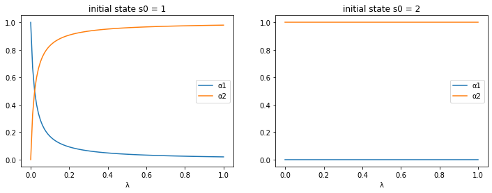
For the specification of the Markov chain in example 3, let’s take a look at how the equilibrium allocation changes as a function of transition probability \(\lambda\).
λ_seq = np.linspace(0, 1, 100)

# prepare containers
αs0_seq = np.empty((len(λ_seq), 2))
αs1_seq = np.empty((len(λ_seq), 2))

for i, λ in enumerate(λ_seq):
    P = np.array([[1-λ, λ], [0, 1]])
    ex3 = RecurCompetitive(s, P, ys)

    # initial state s0 = 1
    α = ex3.wealth_distribution(s0_idx=0)
    αs0_seq[i, :] = α

    # initial state s0 = 2
    α = ex3.wealth_distribution(s0_idx=1)
    αs1_seq[i, :] = α
<ipython-input-3-1395908c3971>:108: RuntimeWarning: divide by zero encountered in reciprocal
  R = np.reciprocal(R)
fig, axs = plt.subplots(1, 2, figsize=(12, 4))

for i, αs_seq in enumerate([αs0_seq, αs1_seq]):
    for j in range(2):
        axs[i].plot(λ_seq, αs_seq[:, j], label=f'α{j+1}')
        axs[i].set_xlabel('λ')
        axs[i].set_title(f'initial state s0 = {s[i]}')
        axs[i].legend()

plt.show()
1.7. Example 4
# dimensions
K, n = 2, 3

# states
s = np.array([1, 2, 3])

# transition
λ = .9
μ = .9
δ = .05

P = np.array([[1-λ, λ, 0], [μ/2, μ, μ/2], [δ/2, δ/2, δ]])

# endowments
ys = np.empty((n, K))
ys[:, 0] = [.25, .75, .2]       # y1
ys[:, 1] = [1.25, .25, .2]      # y2
ex4 = RecurCompetitive(s, P, ys)
# endowments
print("ys = ", ex4.ys)

# pricing kernal
print ("Q = ", ex4.Q)

# Risk free rate R
print("R = ", ex4.R)

# natural debt limit, A = [A1, A2, ..., AI]
print("A = ", ex4.A)

print('')

for i in range(1, 4):
    # when the initial state is state i
    print(f"when the initial state is state {i}")
    print(f'α = {ex4.wealth_distribution(s0_idx=i-1)}')
    print(f'ψ = {ex4.continuation_wealths()}\n')
ys =  [[0.25 1.25]
 [0.75 0.25]
 [0.2  0.2 ]]
Q =  [[0.098      1.08022498 0.        ]
 [0.36007499 0.882      0.69728222]
 [0.01265175 0.01549516 0.049     ]]
R =  [2.12437476 0.50563271 1.33997564]
A =  [[-3.28683339 -1.85525567]
 [-2.9759761  -2.70632569]
 [ 0.11808895  0.14152768]]

when the initial state is state 1
α = [0.63920196 0.36079804]
ψ = [[-0.          0.        ]
 [-0.65616233  0.65616233]
 [ 0.04785851 -0.04785851]]

when the initial state is state 2
α = [0.52372722 0.47627278]
ψ = [[ 0.5937814  -0.5937814 ]
 [ 0.          0.        ]
 [ 0.01787935 -0.01787935]]

when the initial state is state 3
α = [0.45485896 0.54514104]
ψ = [[ 0.94790813 -0.94790813]
 [ 0.39133024 -0.39133024]
 [-0.         -0.        ]]