2 Expectations and Behavior
Rational expectations
The idea of rational expectations has two components: first, that each person’s behavior can be described as the outcome of maximizing an objective function subject to perceived constraints; and second, that the constraints perceived by everybody in the system are mutually consistent. The first part restricts individual behavior to be optimal according to some perceived constraints, while the second imposes consistency of those perceptions across people. In an economic system, the decisions of one person form parts of the constraints upon others, so that consistency, at least implicitly, requires people to be forming beliefs about others’ decisions, about their decision processes, and even about their beliefs.
Why have economists embraced the hypothesis of rational expectations? One reason is that, if perceptions of the environment, including perceptions about the behavior of other people, are left unrestricted, then models in which people’s behavior depends on their perceptions can produce so many possible outcomes that they are useless as instruments for generating predictions. The combination of its two key aspects — individual rationality and consistency of beliefs — has in many contexts made rational expectations a powerful hypothesis for restricting the range of possible outcomes. Another reason for embracing rational expectations is that the consistency condition can be interpreted as describing the outcome of a process in which people have optimally chosen their perceptions. That is, if perceptions were not consistent, then there would exist unexploited utility- or profit-generating possibilities within the system. Insisting on the disappearance of all such unexploited possibilities is a feature of all definitions of equilibrium in economics.[1]
Rational expectations (static)
The two components of rational expectations can be illustrated in the context of a static model of a competitive market. There is a large number of identical firms, each of which chooses its output to maximize , where is an upward sloping cost function. There is a downward-sloping demand function expressing price as an inverse function of total output in the industry, where is the output of the ‘average’ firm in the industry. Each firm takes as given, i.e. is a ‘-taker’ and an ‘-taker,’ and chooses to maximize , which means setting to satisfy the condition ‘price equals marginal cost,’ i.e. . Denote the solution to this problem by , where ‘argmax’ means the maximizing value of . Since via the market demand function, we can also write . The first component of rational expectations thus induces a ‘best-response’ mapping from a given average (or ‘aggregate’) setting for to an optimizing individual choice of .
The second component of rational expectations imposes consistency between individuals’ choices and what their perceptions are of aggregate choices. Because in this simple setting all firms have been assumed identical, imposing consistency amounts to requiring that , so that each firm ends up choosing what it assumes as a -taker (and as an -taker) that the average firm is choosing. By requiring that , we are insisting that each firm, when it acts competitively, has no incentive to deviate from the average setting for that others are assuming in solving their optimum problems.
Thus, a static rational expectations equilibrium is the usual model of a competitive market.
Rational expectations (dynamic)
In the static context just described, a rational expectations equilibrium is a fixed point of the ‘best response mapping’ , a fixed point being a positive real number.[2] However, we often want to study dynamic situations in which individuals choose not one-time actions, but entire sequences of actions. In dynamic contexts, we formulate a rational expectations equilibrium as a fixed point in a space of sequences of prices and quantities, or, equivalently, a fixed point in a space of functions that determine sequences of prices and quantities. We need to define a dynamic analogue of the static best response mapping .[3] This will turn out to be a mapping from a perceived law of motion for the model’s endogenous state variables to an actual law of motion.
Let be a state variable for an individual, for example a stock of capital or labor, and let be the average value of that same state variable over a large number of identical agents, each of whom chooses a contingency plan or decision rule to maximize
subject to
where is an independently and identically distributed random sequence, is a discount factor, and is the mathematical expectations operator. The second equation of (3) is a perceived law of motion or ‘forecasting equation’ for the aggregate state , while the first equation of (3) is an equation for forecasting market price conditional on the value of . The individual solves this problem, taking and as given. The Euler equation for the maximization of (1) with respect to (3) is
where is the partial derivative of with respect to its th argument and is the cumulative distribution function of conditional on aggregate that is induced by the pair of equations (3).[4]
A function that solves this problem is itself a functional of the functions and and the discount factor . The solution of the firm’s optimization problem, , implies that the actual law of motion of the aggregate state is given by . In this way, substituting the condition that the representative firm is representative into the solution of the firm’s optimum problem determines the actual law of motion when the perceived law of motion is . So optimizing behavior and representativeness of the representative firm induce a mapping
from a perceived law of motion to the actual one. A rational expectations equilibrium is a fixed point of the mapping :
Within a rational expectations equilibrium, firms are solving their Euler equation using the equilibrium conditional distribution , that is, the distribution of prices that is induced by (3) with the equilibrium . The two key features of a rational expectations equilibrium are captured by saying that the firm determines its decision by solving an Euler equation (this is the individual optimization part of the definition) using the distribution for the endogenous variable, , that is induced by market clearing and the optimizing behavior of others in the market (this is the consistency of perceptions postulate).
A model of money and prices
These ideas can be illustrated with a rational expectations version of the ‘quantity theory’ about the relationship between prices and the money supply. We use a non-random version of the theory.
We generate a demand for money by assuming that a representative household or money-holder chooses its level of nominal balances to carry over from time to time to maximize the objective function
where we assume that . Here is a parameter that measures resources now available to consume or save in the form of real balances, while is a parameter that measures resources that will become available next period. The objective function describes how the money-holder weighs the sacrifice involved in holding units of currency this period, which costs him units of goods for each dollar held from this period to the next, against the additional units of goods that he expects this dollar will command next period. The money-holder chooses , taking as given the current price level and what he expects the price level will be next period, . The maximizing choice of determines the money demand function[5]
To make (8) operational requires a theory of how the expectation is formed. We can build in rational expectations as follows. Suppose that the supply of money is exogenously set by the government to follow the law of motion
for all time . Suppose further that the household observes the money supply at , and that it believes that the price level is related to the money supply via the relationship
where are constants that summarize the household’s expectations or beliefs. We assume that these parameters take values for which the price level is always positive for any positive money supply for any time . In particular, we assume that . Suppose also that the household knows the value of in the law of motion for the money supply, and that it uses the law of motion for the money supply and equation (10) to forecast the price level next period as
Substituting this equation into (8) and (10) and rearranging gives
Equation (12) shows a common feature of models in which expectations about the future play a role: the demand for money can be regarded as depending on the supply. This dependence emerges because current demand depends on expectations about future price levels, and future price levels are believed to depend on future values of the money supply, which are related to the current money supply by the law of motion (9). Equation (12) determines the demand for money as a function of exogenous variables known at , namely, the money supply.
To compute a rational expectations equilibrium, we set the demand equal to the supply, in (9), and solve the resulting ‘functional equation’:
This equation has a function of on both the right and left sides. We have a rational expectations equilibrium if these two functions are equal, which occurs only under the conditions
When the parameters assume these values, the price level obeys the law
When prices follow this process, the household’s expectations about the price level are given by , and always turn out to be correct. Notice how the parameter from the law of motion of the money supply enters the equation (16) which shows how the price level depends on the money supply.
The equilibrium is not unique. For any constant we have an equilibrium. Since , for any equilibrium with , prices have a component that is unrelated to money supply behavior and that is growing exponentially at rate . There is one equilibrium (the one with ) in which the price level is proportional to the money supply. All of the (continuum of) other equilibria have the price level rising in what is referred to as a purely speculative ‘bubble.’ This is one among many examples in which rational expectations equilibria are not unique, in which case ‘fundamentals’ are incapable by themselves of determining market prices and quantities.[6],[7]
Extending back to Ricardo and Wicksell, there is a tradition in macroeconomics of using models with indeterminate equilibria to criticize the arrangements or operating procedures that the modeller shows to cause the indeterminacy. We turn briefly to an indeterminacy that has haunted international monetary theory.
Another indeterminacy
We can adapt the above model of money and prices to describe an indeterminacy in a theory of exchange rates in a world of fiat currencies.[8] We now assume that (8) governs the total demand for two currencies, which are available in total supplies and , respectively, at time . We also assume that the two currencies are perfect substitutes so long as their rates of return are equal. The supplies are governed by the laws of motion
Let be the price level denominated in units of currency , . Let be the expected price level in units of currency . We suppose that the two currencies are always expected to appreciate at the same rate, so that
a condition that makes holders of currency indifferent about which currency they hold. (People’s indifference about the composition of their money holdings will be the key feature rendering the exchange rate indeterminate.)
Suppose that people believe that the price levels , are determined by
where is a constant exchange rate. Equations (18), (19), and (21) imply that forecasts of the price levels are made according to
Notice that (21) and (23) imply that (19) is satisfied and is expected to remain satisfied. Substituting these into the demand for money, denominated in units of currency 1, namely, , gives
For equilibrium, we require that , i.e., the demand for currency denominated in units of currency 1 equals the total supply. This determines a functional equation,
whose solution is
These equations are remarkable because they leave the exchange rate unrestricted. If these equations have a solution for one , then they have a solution for any other . Furthermore, the formulas for do not involve the exchange rate .
Besides being of substantive interest, such models of monies, prices, and exchange rates provide examples of some important methodological issues involving the construction and application of rational expectations models. First, notice how an equilibrium was constructed by using a ‘guess and verify’ or ‘undetermined coefficients’ method. In each example, we guessed at an expectations-generating function of a particular form (linear) with free coefficients, and then computed the values that those coefficients would have to take if expectations were to be rational in light of the structure of the complete model. This solution procedure is silent about how the agents being modelled are supposed to have acquired the beliefs attributed to them. Furthermore, this solution procedure works only in very special cases (essentially only in linear models). In more general settings, the model builder needs some other method for finding an equilibrium.
Second, these are examples of a class of rational expectations models in which equilibria are not unique. There are multiple systems of beliefs, indexed by the parameter in the money model and by the parameter pair in the exchange rate model, that are consistent with rational expectations. Rational expectations alone is not a sufficiently restrictive principle to determine outcomes. If we want to apply such a model to interpret economic time series, some principle other than rational expectations must be used to choose among the possible equilibrium outcomes.[9],[10]
Computation and ‘stability’ of equilibrium
Static stability and ‘adaptive expectations’
We are confronted with the following two distinct but, in practice, related questions. First, given the parameters of a model, how might an equilibrium actually be computed by economists interested in applying the model; and second, supposing that the market ‘starts’ from some non-equilibrium quantity , can we describe an ‘adjustment mechanism’ that under particular circumstances would eventually converge to equilibrium?
For our static model, a starting point for many computational schemes is the following ‘relaxation algorithm’:
or
where is a so-called ‘relaxation parameter,’ and is the estimate of the equilibrium value at the th iteration. For some assumptions about the best response mapping , there exists a for which this scheme converges to the equilibrium value .[11]
In this iterative scheme, can be loosely interpreted as an ‘expected’ or ‘anticipated’ value[12] of at iteration , while is taken to be the ‘actual’ value at iteration . Each iteration of the scheme adjusts the expected value towards the actual value by an amount determined by . ‘Stability’ has sometimes been taken to be the requirement that such a scheme converges.
Suitably reinterpreted, this iterative scheme provides a basis for Friedman’s and Cagan’s concept of ‘adaptive expectations.’[13],[14] The equilibrium of the static model describes a timeless situation, or else a situation in which nothing changes with the passage of time. One motivation behind the idea of ‘adaptive expectations’ was to ‘tack dynamics’ onto a static model by replacing iteration step by calendar time , and to take the resulting equation as a description of how agents form expectations about from one period of time to the next. With replaced by , equation (31) can be rearranged into the equivalent forms
or
which are two alternative forms of adaptive expectations. In their studies of hyperinflation and consumption, respectively, Cagan and Friedman used their adaptive expectations scheme to describe the evolution of people’s expectations in real time. In their studies, the expectations-generating function (33) played a key role in determining system dynamics. Their work showed that using (33) with helped them to fit and to interpret the data in terms of dynamics largely driven by expectations formation. Cagan and Friedman left open the question of why people would choose to form expectations according to (33).[15] Friedman and Cagan took to be a free parameter of their models, the single free parameter describing beliefs.
John F. Muth wanted to eliminate as a free parameter. Muth sought simple dynamic environments in which it would be a good idea to form expectations as in (33). He structured his search as an ‘inverse optimal prediction’ problem, seeking a univariate stochastic process for with the property that the linear least squares forecast of for at least some horizon would be of the form (33). He found that (33) would be the optimal forecast of over any horizon if and only if evolved according to a univariate stochastic process described by
where is a martingale difference sequence. This is the only environment for which the forecasting scheme (33) delivers unimprovable forecasts, given the information that the rule uses. In Muth’s vision, the forecasting scheme (33) inherits its one parameter from the stochastic process (34) actually governing the process being forecast.[16] Muth’s work was the first application of the idea of rational expectations to find restrictions across a forecasting scheme and an economic–statistical environment in which that scheme was to be used; it led subsequent researchers[17] to think of the forecasting scheme itself as the object in terms of which the equilibrium of a dynamic model is to be defined.[18]
Computation of dynamic equilibrium
In moving from our static example to the dynamic one, we did something quite different from simply tacking the Cagan–Friedman adaptive expectations scheme onto the static model: we changed the space of objects in terms of which we defined an equilibrium. Whereas in the static model the equilibrium was defined as a real number representing the quantity of output in the industry, in the dynamic model the equilibrium was defined as a function mapping past values of industry output and random disturbances into future values of industry output. In effect, we defined the equilibrium in terms of an expectations-generating scheme that is optimal given the economic environment.
The adaptive expectation scheme (33) is a particular example of a distributed lag expectations scheme that maps a history into an anticipated value of . Muth’s (1960) purpose was to find a particular stochastic environment expressing as a function of the history and additional random factors ,
and for which Cagan and Friedman’s scheme would be an ‘optimal’ distributed lag. Normally, we are in an opposite situation to the one Muth studied: we start from a description of the environment, and want to find an function that is ‘self-generating.’
One way to think about computing equilibrium in a dynamic model is to consider iterations mapping estimates of the function into new estimates. Corresponding to (31), we have the adaptive scheme
or
where is again a relaxation parameter. Equation (37) is a scheme for revising entire (expectations-generating) functions in response to discrepancies between their predictions and actual outcomes. We shall meet such schemes again.
Bounded rationality
Behavioral aspects of rational expectations
The idea of rational expectations is sometimes explained informally by saying that it reflects a process in which individuals are inspecting and altering their own forecasting records in ways to eliminate systematic forecast errors. It is also sometimes said to embody the idea that economists and the agents they are modelling should be placed on an equal footing: the agents in the model should be able to forecast and profit-maximize and utility-maximize as well as the economist — or should we say the econometrician — who constructed the model. These ways of explaining things are suggestive, but misleading, because they make rational expectations sound less restrictive and more behavioral in its foundations than it really is. It was not the way that Muth originally defined rational expectations, and it misses key features of the way rational expectations models are implemented in practice.
Rational expectations equilibrium as a fixed point in a mapping from perceived to actual laws of motion typically imputes to the people inside the model much more knowledge about the system they are operating in than is available to the economist or econometrician who is using the model to try to understand their behavior. In particular, an econometrician faces the problem of estimating probability distributions and laws of motion that the agents in the model are assumed to know. Further, the formal estimation and inference procedures of rational expectations econometrics assume that the agents in the model already know many of the objects that the econometrician is estimating.
Artificial agents who act like econometricians
Herbert Simon and other advocates of ‘bounded rationality’ propose to create theories with behavioral foundations by eliminating the asymmetry that rational expectations builds in between the agents in the model and the econometrician who is estimating it. The idea of bounded rationality might be implemented by requiring that the agents in the model be more like the econometrician in one or more of several ways. The agents might be like ‘classical econometricians,’ who are sure of their model but unsure of parameter values; they might be like ‘Bayesian econometricians,’ who are unsure of their models and parameter values but can say how they are unsure; or they might be like many practicing macroeconomists, who are unsure even about whether they want to proceed as if they are classical or Bayesian econometricians.
We can interpret the idea of bounded rationality broadly as a research program to build models populated by agents who behave like working economists or econometricians. To lay out the road ahead, it will be useful to say a little more about what we mean by ‘behave like economists.’
Practice of economics
Like any science, economics has these parts: a body of theories (self-contained mathematical models of artificial worlds); methods for collecting or producing data (more or less error-ridden and disorganized measurements); statistical methods for comparing a theory with some measurements; and a set of informal procedures for revising theories in the light of discrepancies between them and the data.[19] The intent of the ‘bounded rationality’ program is to work the methodology of science doubly hard because, in attempting to understand how collections of people who make decisions under uncertainty will interact, it will use models that are populated by artificial people who behave like working scientists.[20] These artificial people process data and make decisions by forming and using theories about the world in which they live. In other words, the economist will assume that he is modelling sets of people whose behavior is determined by the same principles that he is using to model them.[21] Rational expectations is an equilibrium concept that at best describes how such a system might eventually behave if the system will ever settle down to a situation in which all of the agents have solved their ‘scientific problems.’
Partly because it focuses on outcomes and does not pretend to have behavioral content, the hypothesis of rational expectations has proved to be a powerful tool for making precise statements about complicated dynamic economic systems. In game theory and general equilibrium theory, we have learned how to impose the two hypotheses of individual rationality and consistency of beliefs in more and more varied and interesting contexts.
The idea of building dynamic theories with behavioral foundations by modelling agents as economists or scientists is intuitively attractive and consistent with the way many of us see the world. But implementing this vision has proved difficult for a variety of reasons, a paramount one being that we don’t really have a tight enough theory or description of how economists or other scientists learn about the world. And within economics and other sciences, there are important differences in how different practitioners go about the process of discovery.
Artificial intelligence
Thus, an impediment to implementing bounded rationality as a viable research program is the wilderness of possibilities into which it seems to lead us. Precisely how are we to go about building models populated by agents who in some sense are behaving ‘like us scientists’? A number of economists are answering this question by combing the recent literature on artificial intelligence as a source of methods and insights. The past fifteen or so years has seen an explosion of work designed to create artificial systems or ‘brains’ that adapt and learn. Some of these methods embody sensible versions of at least aspects of what we might mean by ‘behave like a scientist.’ The process of borrowing methods from this literature to create economic models has already led to a variety of models of bounded rationality. The remainder of this book will be devoted to surveying parts of the literature on artificial intelligence and to describing how they are related to methods that macroeconomists might already know and use or might eventually come to use.
Questions and payoffs
In the methodology of positive economics of Milton Friedman (1953), economic models are judged by how the outcomes that they predict match data measuring the economy. From the standpoint of this methodology, the behavioral emptiness of rational expectations is neither virtue nor defect. To justify the research effort called forth by the bounded rationality program, we require some prospective payoffs in terms of concrete questions that rational expectations models are not likely to be capable of answering. What are these questions, and where are the likely payoffs?[22],[23]
Equilibrium selection
Rational expectations models sometimes have too many equilibria.[24] When there are multiple equilibria, it means that the physical description of the economy together with the notion of equilibrium are not sufficient to pin down a unique predicted outcome. Many rational expectations models have unique equilibria, but enough of them have multiple equilibria that researchers in game theory and general equilibrium theory have turned to models of bounded rationality somehow to reduce the multiplicity of equilibria. In these contexts, the motivation for embracing a behavioral theory of out-of-equilibrium behavior is the hope that, by studying plausible processes of adapting to out-of-equilibrium behavior, we will find that only particular types of equilibria are possible limit-points of out-of-equilibrium behavior. We shall encounter several more or less successful examples of work motivated in this way.
New sources of dynamics
While rational expectations has proved to be a powerful method of generating rich and interesting dynamics in various contexts, there are particular areas in which the outcomes that it predicts are sharp but very difficult to reconcile with observations. A leading example is from finance, where a powerful ‘no trade’ theorem characterizes a class of situations in which diversely informed traders are so efficiently extracting information from equilibrium prices that literally no volume of trade can occur in any equilibrium. To explain volume data from financial markets, one needs a model for which the no-trade theorem fails to hold. For rational expectations models, it has proved very difficult to produce a compelling rational expectations model that breaks the no-trade theorem. This has led researchers such as Princeton’s Harald Uhlig and Stanford’s John Hussman to begin studying models of asset markets populated by boundedly rational differentially informed agents.
This is but one example of a class in which it seems that sticking with rational expectations might not give us enough flexibility to model all of the dynamics in the data, and in which resorting to adaptive models may help us. Even in macroeconomics within the rational expectations tradition, models are routinely used in ways that are inconsistent with rational expectations.
Analyses of ‘regime changes’
Rational expectations models have been used to make statements about the consequence of regime changes, a term that is often used in a way that precludes its being consistent with rational expectations. I have in mind work that characterizes a government policy rule as an arbitrarily given state- and time-contingent policy rule, then computes a rational expectations equilibrium under two different such policy rules. Often the first rule is a ‘pre-reform’ rule meant to describe the government’s behavior historically, while the second rule is what the modeller intends as an improved rule. The change in outcomes across hypothetical economies operating for ever under these different rules is then used to predict what would occur if the proposed government policy rule were to be adopted at some future date.
This way of generating predictions is inconsistent with rational expectations because, by comparing equilibria of different economies, it predicts what would happen if at some time in the future the government were to deviate from what it had initially been assumed to have for ever committed itself to.[25]
Under rational expectations, if the government was to have had the option of changing its behavior at future points in time, the agents in the model should have been given the opportunity to take this possibility into account. That is, if the government were really choosing sequentially and not once-and-for-all at time 0, under rational expectations the response of ‘the market’ would change in ways that depend precisely on the government’s motives and the dates at which it is given the opportunity to choose. Under a thorough application of rational expectations, if the government really has the option to default from its time 0 plan, that option should be described and the initial equilibrium recomputed under a set of beliefs for private agents about how likely it is that the government will choose that option.
Despite the fact that they are inconsistent with rational expectations, these types of regime change experiments have been a principal use of rational expectations models in macroeconomics. One example is the analysis of the ends of hyperinflations in terms of monetary and fiscal policy ‘regimes.’[26] To analyze the ends of hyperinflations, models of money like the one described above have been used to compute rational expectations equilibria under two alternative full-commitment monetary-fiscal regimes. A first, ‘pre-reform,’ regime has permanent large government net-of-interest deficits that are permanently financed by high rates of printing government-issued currency. A second, post-reform, regime has a government budget that is permanently balanced in present value, and no currency is ever created to finance government deficits. These models predict permanently high rates of inflation in the first regime, and no inflation in the second regime.
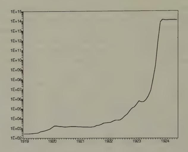
Figure 1:Wholesale Prices in Germany, 1919–1924
This comparison has been used to interpret data like Figure 1 and Figure 2, which show the abrupt stabilizations of price levels at the ends of hyperinflations in Germany and Austria after World War I. In each country, the end of the hyperinflation coincided with a set of government actions that seem consistent with implementing a switch from the first regime to the second regime that I have just described. That the price stabilizations occurred so rapidly perhaps provides some reason for thinking that we don’t make much of an error by ignoring the possibility that the prospects of a regime change occurring should really have been built in when analyzing the initial regime.
Retreating from rational expectations
The hyperinflation example is one in which not insisting on consistency with rational expectations is justified as a short-cut that, for the question at hand, appears to cost little. There is another class of historical examples in which giving up on rational expectations at some (shrewdly chosen) point seems essential for understanding what is going on. Understanding the arrangements and disturbances that led to the onset of the Great Depression is a case in point.[27] I shall describe two competing stories about the onset of the Great Depression, each of which uses many elements of rational expectations, but essential to each of which is a backing off of rational expectations at some level.
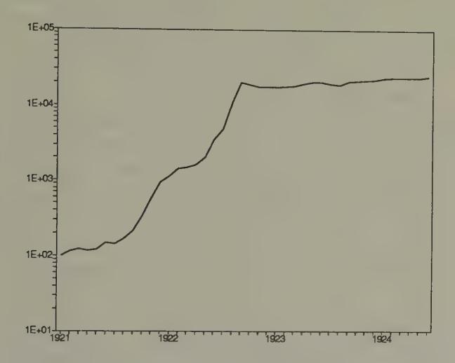
Figure 2:Retail Prices in Austria, 1921–1924
Here is the first story. For fifteen years after its inauguration in 1914, the Federal Reserve System was widely regarded as having solved the problem of financial fragility that had been manifested earlier in recurrent panics and temporary suspensions of convertibility of banks’ deposits into gold. The Federal Reserve Act replaced the informal mechanisms that had emerged to cope with those problems[28] with a system of Federal Reserve banks that was instructed to provide enough ‘elasticity’ to the currency supply to avert panics. The Federal Reserve Act assigned two duties to the Federal Reserve System: first, to act as a ‘lender of last resort’ in times of general financial stringency and second, to maintain the gold standard, that is, to assure that Federal Reserve notes were convertible to gold on demand. The first assignment was designed to stop panics; the second was designed to implement a commitment to price stability.
Because the Federal Reserve System had no powers to tax, it was not feasible for it alone, without assistance from the Treasury, to carry out both of these assignments in all possible states of the world. To maintain a gold standard under the system of fractional gold reserves then in place, the government had to stand ready to tax enough to ‘service’ the debt that it had issued or insured, in this case in the form of Federal Reserve notes and liabilities convertible into them. If it had no powers to tax, or to induce other agencies to tax to support its assignments, the central bank could assure convertibility into gold only by running a version of a 100 percent reserves policy. This would entail preventing banks and other financial institutions from intermediating risky private indebtedness in exchange for notes and deposits that claimed to be convertible into gold. In that way, the Federal Reserve could have maintained the convertibility of its own notes, although in doing so it would resign its duty to maintain an elastic currency and so give up functioning as a lender of last resort for banks who were in the business of intermediating risky liabilities.
If it had been relieved of the assignment to maintain convertibility into gold, it would have been feasible for the Federal Reserve to act as a lender of last resort, by appropriately managing timely depreciations of the currency against gold.[29] In effect, relieving the Federal Reserve of the assignment to maintain convertibility with gold would have given it a tax (the ‘inflation tax’) with which to finance its lender-of-last-resort (or bailout) activities.
So it was not feasible for the Federal Reserve to carry out these two assignments. Nevertheless, during the 1920s many people talked and acted as though they believed that the Federal Reserve could and would carry out those assignments; and for a string of years the system seemed to be working. Too many bankers and depositors regarded the system as sound, and failed to recognize that the scheme was infeasible in some states of the world. Instead, bankers and depositors responded as though they were operating under a form of unpriced implicit deposit insurance (for what else does ‘lender of last resort’ mean?) and they responded appropriately. Operating in their shareholders’ interests, banks undertook riskier projects than they would have in the absence of implicit deposit insurance, thereby exposing the system to increased risk and bringing closer the day when the Federal Reserve might be called upon to lend in such volume as to jeopardize its commitment to the gold standard. That situation arose in 1931, when the banks and depositors learned that it was not feasible for the Federal Reserve both to act as a lender of last resort and also to keep the system on gold. Until 1933, when Roosevelt engineered a big depreciation in terms of gold, the Federal Reserve met its gold standard commitment at the expense of its lender-of-last resort function. Banks’ and depositors’ failure fully to ‘see through’ the Federal Reserve System’s infeasible promises set in motion a process that led to massive financial failure.
Notice how this story uses bits and pieces of rational expectations reasoning, but suspends rational expectations beyond a point. The story has people ‘look several steps ahead,’[30] but has them stop well short of seeing through the entire mechanism.
There is an alternative story, which backs off from rational expectations in perhaps a more obvious way than does the first one. Written into the Federal Reserve Act was a version of the ‘real bills doctrine,’ according to which the Federal Reserve banks were instructed freely to discount at low interest rates high-quality (i.e. relatively risk-free or ‘real’) evidences of commercial indebtedness as a device to provide an ‘elastic currency.’ The sense of the ‘real bills’ policy was to integrate money and credit markets, by making the supply of currency depend on the state of credit markets. There is evidence that during the 1920s the Federal Reserve System was operating under a version of a real bills regime.
The real bills regime has long been criticized by advocates of an alternative set of rules for running a central bank which can be described as a ‘quantity theory’ regime. The quantity theory regime aims to separate the money market from the credit markets, in order to prevent fluctuations in the supply and demand for credit from impinging on the price level. Because borrowers are cut off from currency holders as potential lenders, under a quantity theory regime there is typically less elasticity of the currency supply and a higher level of interest rates than under a real bills regime. The levels of equilibrium interest rates and asset prices depend on the monetary and intermediary-regulation regime in place.[31]
Here, then, is our second story. During the 1920s the Federal Reserve ran a real bills regime, which participants in the economy assumed was a full-commitment, everlasting policy regime. But starting around 1930,[32] the Federal Reserve abruptly began to administer a quantity theory regime. This entailed an upward movement of real interest rates, causing all sorts of assets to suffer capital losses, and turning many ‘good loans’ into ‘bad loans.’
The structure of our second story shares with our hyperinflation example the key feature that the prime mover is an exogenous change in government policy. However, in the present story, it is essential that the government’s change in policy and its consequences were not anticipated beforehand.
These stories should not be confused with hard analyses, and are intended only to indicate how using rational expectations models in ‘impure’ ways that do not fully impose the two key features of rational expectations (individual rationality and consistent expectations) provides ample — maybe too much — freedom to explain some observations that are difficult to explain if we remain thoroughly faithful to rational expectations.
New optimization and estimation methods
There is another lode of likely benefits from studying the artificial intelligence literature, but these have less to do with finding new ways of modelling the adaptive behavior of economic agents and more to do with finding new ways of conducting our own business as economists. As practicing economists, we are always on the lookout for new ways of solving optimization, estimation, and numerical analysis problems. The literatures on artificial intelligence and neural computing are full of ideas that are potentially applicable to our problems as researchers. In the spirit of the bounded rationality research program, which is really to put the economist and the agents in his model on an equal behavioral footing, we expect that, in searching these literatures for ways to model our agents, we shall find ways to improve ourselves.
Plan of the book
The elementary object of analysis in rational expectations models and models of bounded rationality is a collection of decision rules, namely, functions mapping people’s information into decisions. Rational expectations restricts those decision rules by adopting the two assumptions of individual optimization and consistency of perceptions. Bounded rationality drops at least the second of these assumptions, and replaces it with heuristic algorithms for representing and updating decision rules. Students of bounded rationality are therefore in the market for good ways of encoding decision rules and updating them as new information flows in.
The next two chapters briefly survey the two spots where researchers have gone prospecting for the algorithms needed to populate models with boundedly rational artificial agents. The first place is an old literature on statistics and econometrics, while the second is a newer literature on networks and artificial intelligence.
After surveying some of these methods and describing their relationships in Chapters 3 and 4, in Chapter 5 we put some of the methods to work on five examples. Then Chapter 6 describes two laboratory experiments that have been performed on versions of one-currency and two-currency versions of the model of money and prices described above; the authors of both of these experiments used adaptive algorithms to interpret their results. Chapter 7 sums things up.
The first use of the term ‘rational expectations’ that I know is by Hurwicz (1946, p. 133), who did not define the term, but used it in discussing ways of modelling the behavior of a single firm facing an unknown distribution of future output prices. Muth’s (1961) definition emphasizes the second aspect of the concept, consistency of perceptions. Hurwicz (1951) used both elements of the concept of rational expectations, though he did not use the term in his discussion of econometric policy evaluation procedures.
Or, in random models, a random variable.
The example in this section is close to that of Lucas and Prescott (1971).
This is a version of the demand function for money used by Phillip Cagan (1956) to study hyperinflations. The objective function that we have attributed to the household corresponds to one that is often used in versions of Paul Samuelson’s (1958) overlapping generations model; for example, see Neil Wallace (1980).
Blanchard and Watson (1982) have pointed out that there are many other equilibria of a stochastic version of this model, formed by regarding as the mathematical expectation of conditioned on information known at time . These equilibria are identical to (16) except that now in (16) is replaced by a stochastic process , where is any martingale.
In computing a rational expectations equilibrium, we are solving for the parameters , , that determine people’s beliefs (through (10)) as functions of other parameters in the model. When an equilibrium is unique, ‘beliefs’ contribute no free parameters to the model. When equilibria are not unique, as in this example, some of the free parameters index beliefs.
Versions of this result are due to Russell Boyer (1971) and Kareken and Wallace (1981).
King, Wallace, and Weber (1992) build a model in which many stochastic paths of exchange rates are equilibria.
In a class of overlapping-generations models with free currency substitution, Manuelli and Peck (1990) show that the only restriction that equilibrium imposes on the exchange rate is that it conform to a bounded martingale. They construct various types of equilibria, some depending on long histories of ‘fundamentals’ that are used in effect to synthesize innovations used to drive martingale exchange rate fluctuations. In the Manuelli–Peck context, it is hard to imagine exchange rate fluctuations that are ‘too volatile’ either in the sense that they are inconsistent with equilibrium or in the sense that their volatility reflects (Pareto) bad welfare outcomes.
One set of sufficient conditions amounts to requiring that an associated differential equation have a unique rest point and that it be stable about it.
In a loose ‘psychological’ sense, not in the sense of mathematical expectation.
‘Adaptive’ mechanisms will be described throughout this book. At this point, the phrase just refers to schemes of the form (31) in which an estimate of an object is adjusted in a direction to diminish the discrepancy between it and the object. By varying the ‘space’ in which the object under study resides and sometimes also by making a decreasing function of the iteration number , many different adaptive mechanisms will have representations like (31).
Milton Friedman credits A. W. Phillips as having suggested the adaptive expectations formulation to him.
Friedman took up the question later (Friedman 1963).
In the context of Cagan’s (1956) model, Sargent and Wallace (1973), Christiano (1987), and Hansen and Sargent (1983) studied multivariate versions of Muth’s inverse optimal prediction problem, and found joint processes for money and prices that make optimal an adaptive expectations scheme for forecasting prices. For the permanent income example studied by Muth, Sargent (1987, ch. XIII) provides a different solution of the inverse optimal predictor problem that rationalizes Friedman’s specification.
See Lucas and Prescott (1971) and Brock (1972).
Muth wanted to deduce restrictions on expectational distributed lag models of the general form , where is interpreted as a forecast of conditioned on observations through , and is the polynomial in the lag operator . In effect, Muth proposed restricting to be the systematic part of an autoregressive representation of . Grandmont (1990) has formalized and extended a pre-Muthian set of restrictions on . He proposes that for a fixed set of frequencies , the forecasting scheme should be able perfectly to forecast periodic sequences . This leads to the restrictions , for the frequencies chosen. Imposing these restrictions at frequencies determines . (For example, for frequency , the restriction is , which is the famous ‘sum of the weights equals unity’ restriction.) Early work in the rational expectations literature (e.g. Lucas 1972; Sargent 1971) described the conflict between this way of restricting distributed lags and Muth’s.
In economics, procedures for revising theories in light of data are typically informal, diverse, and implicit.
Primo Levi said ‘a chemist does not think, indeed does not live, without models ...’ (The Periodic Table: Levi 1984, p. 76)
Such a system can contain intriguing self-referential loops, especially from the standpoint of macroeconomic advisors, who confront the prospect that they are participants in the system that they are modelling at least if they believe that their advice is likely to be convincing.
Niels Bohr said, ‘It is wrong to think that the task of physics is to find out how nature is. Physics concerns what we can say about nature.’ This quotation is from the biography of Bohr by Abraham Pais (1992).
I exclude from the following list of potential payoffs the aim of building psychologically deeper or ‘more realistic’ models of the way people behave. The cognitive psychologist Lawrence Barsalou (1992, p. 9) points out that ‘Cognitive constructs — as I will call internal constructs in cognitive psychology — typically do not represent conscious mental states. Instead, they typically represent unconscious information processing.’ To the extent that we think that economic decision-makers are acting consciously, Barsalou warns us not to expect too much help from his field at the present time.
David Kreps (1990) discusses issues involving equilibrium selection in games. Many of the issues in this essay, and some of the viewpoints, are identical to ones discussed by Kreps in related contexts.
A modeller can solve a Ramsey problem by finding the government policy rule that, within a class, optimizes an objective function that the modeller attributes to the government, typically a weighted average of the utilities of the agents in the model. In this work, commitment by the government is modelled formally as selecting a state- and time-contingent policy rule at time 0, and then never reconsidering any decision. Using models to compute Ramsey policies is consistent with rational expectations, at least under this particular assumption about the timing of government decisions, because it builds in optimizing behavior on the part of all agents and imposes a consistent set of expectations across agents.
The description in the text fits my own work on the ends of big hyperinflations (Sargent 1986, ch. 3), but misses some influential analyses of hyperinflations. Flood and Garber (1983) and LaHaye (1985) have focused on the effects during the hyperinflation of speculation about when a stabilization will occur. Also, see Hamilton’s (1989) model of regime switches.
The very speculative remarks in this section are based on recollections of discussions at the Federal Reserve Bank of Minneapolis with Neil Wallace.
See Friedman and Schwartz (1963, pp. 156–68).
See Beers, Sargent, and Wallace (1983).
Thus, the banks are assumed to understand the workings of a ‘Modigliani-Miller theorem,’ which describes the incentives that the system seems to have given them for increasing the risk in their portfolios to the benefit of their shareholders. See Kareken and Wallace (1978) and Merton (1978). But the banks, investors, and creators of the Federal Reserve are assumed not to foresee (or care about?) the system-wide consequences of their behaviors.
See Sargent and Wallace (1982) and Bruce Smith (1988) for comparisons of the quantity theory and real bills regimes.
Perhaps partly due to the death of Benjamin Strong.