3 Data Structures
Statistics and bounded rationality
Statistics studies methods of making inferences and decisions when we aren’t sure what is happening. For economists, statistics has long been the place to go prospecting for hypotheses to understand how people behave under conditions of uncertainty and ignorance. It must be our starting place, because we propose to make our agents even more like statisticians or econometricians than they are in rational expectations models.
The purpose of this chapter is to review the workings of that centerpiece of econometrics, least squares regression, and how in many contexts it can be implemented recursively. This review will set the stage for the following chapter on neural networks and artificial intelligence, material that is less familiar to most economists, but which we shall see just implements recursive least squares in various ingenious contexts. In this chapter and the next we shall be looking for devices to hand over to the boundedly rational agents that will be created in Chapter 5.
Representation and estimation
From statistics, economists have borrowed and adapted a set of methods for describing and interpreting relationships within data sets. The task of description has fruitfully been subdivided into two logically distinct but interrelated pieces: representation and estimation. Representation of a relationship means positing a mathematical model that is assumed to have generated the data.
Usually, the data are taken to be a random sample drawn from a particular probability distribution, and the task of representation is to select a tractable model describing that probability distribution, typically in terms of a small number of parameters. The mathematical model chosen to represent the data is sometimes called the ‘data generating mechanism.’ The job of representation is ‘purely mathematical’ and in itself involves no use of statistical inference. Statistical methods are used to estimate the free parameters of the mathematical model, on the basis of the data set under study.
This chapter briefly describes some of the data-generating mechanisms that economists widely use, and also the sorts of procedures that they use to estimate the parameters of those models. My purpose is to convey the flavor of these data-generating mechanisms and statistical procedures, and to set the stage for our subsequent comparisons with neural networks.[1]
Two versions of the linear regression model
Population version
Linear regression, a pillar of econometrics, is a tool for summarizing the linear structure of a vector of random variables. We have a probability distribution function for where is a scalar and is a vector. We assume that the probability distribution has well defined first and second moments. We want to represent the probability distribution in the form
where approximates in the sense that is as small as possible in the mean square norm , where is the mathematical expectation. The object is to select to minimize .
The first-order condition for minimization of is , where . Thus, the (population) least squares satisfies the orthogonality condition
or
Notice that the population least squares regression coefficients is a mathematical object defined in terms of the population second moments of the distribution . By virtue of the orthogonality condition (2), because , the least squares regression represents as the sum of a linear function of and a piece that is orthogonal to .
The sample version
We have a sample of observations , drawn from the distribution . Everything that we know about the moments of is contained in the sample . From these data, we want to estimate the unknown value of in the model
We can accomplish this by replacing expectations with sample means in formula (3); namely, we use
This is ‘ordinary least squares.’
Vector autoregressions
Following the advice of Sims (1980), macroeconomists often use systems of linear regressions, with one equation for each variable being studied, to represent the dynamics within a collection of economic time series. Each variable is regressed against lagged values of itself and all of the other variables in the model.
Let be an covariance stationary stochastic process (i.e., one for which the vector of means is independent of time and the matrix covariances are well defined and independent of calendar time ). For convenience, assume that . Under particular conditions, such a process has the autoregressive representation
where is an vector of least squares residuals or ‘innovations’ that satisfies the extensive orthogonality conditions
This model is called a vector autoregression. The force of the extensive orthogonality conditions in the last equation is to decompose into a piece , which is linearly predictable from past values of the vector process itself, and a part , which cannot be predicted linearly from past ’s (i.e., it is orthogonal to each element of past ’s). The matrices of autoregressive coefficients are determined by the normal equations
which are equivalent with the least squares orthogonality conditions.
The vector autoregressive representation is a workhorse. Following the lead of Sims and Litterman, it is often used to represent systems of interrelated time series for the purposes of describing their dynamic structure and forecasting them. In constructing our models of economic agents, economists often describe their beliefs about the dynamics of the environment in terms of a vector autoregression. We use vector autoregressions to formulate our own forecasting problems, and often model economic actors as doing the same.
Estimation of vector autoregressions
If enough data were available, vector autoregressions could be well estimated by applying ordinary least squares, equation by equation. But economists usually don’t have enough data to use ordinary least squares, so Sims and Litterman have shown how to use modified versions of least squares. I postpone discussing why in practice they deviate from using ordinary least squares in its unadulterated form.
Stochastic approximation
Robbins and Monro (1951) considered the problem of finding a value of a vector that solves the equation
where is a function that is decreasing in , and is a sequence of vectors of random variables drawn from some sequence of probability distributions where . It is assumed that
(a) either a sample has been generated by ‘nature,’ or one can be generated by simulation; or
(b) the function can be evaluated for the generated and any admissible candidate .
The stochastic approximation algorithm for computing a sequence of estimates of the value that solves (9) is
where is a nonincreasing sequence of positive numbers satisfying
Robbins and Monro (1951) and their followers described conditions under which
where solves either (in the case that is drawn from a distribution that is stationary) or (in the case that is asymptotically stationary).[2]
It has been discovered that the limiting behavior of a sequence determined by stochastic difference equation (10) is described by an associated differential equation,
where is the expected value of , evaluated with respect to the asymptotic stationary distribution of .
A heuristic justification for (13) notes that for large values of algorithm (10) is approximated by
where replacing in (10) with an expected value at a fixed , namely, , is justified by observing that, for large , , and that the randomness in will make its variation large relative to the variation in . Use the time transformation to write this differential equation as
which is the ordinary differential equation (13) to be used to approximate the limiting behavior of in (10).
A recursive formulation of the least squares estimate of the mean provides a simple example of stochastic approximation. The least squares estimate is the sample mean . Subtracting the sample mean at from both sides of this formula and rearranging gives
which is in the form of (10) with the ‘gain’ . The usual initial condition for this equation is .[3],[4]
Recursive least squares
The stochastic approximation algorithm can be used to implement the least squares formulas recursively. Suppose that we set , , , and
Then the stochastic approximation scheme becomes
Starting from appropriate initial conditions , this is a method for calculating (5). Alternatively, it can be interpreted as a Bayesian procedure for updating estimates starting from a prior distribution .
Least squares as stochastic Newton procedures
Sometimes we want to minimize the function with respect to . The gradient descent method is iteratively to choose according to
for some positive step-size sequence . Newton’s method is to choose according to
For the regression problem, we choose and . Since and , a gradient descent and Newton’s method become, respectively,
Notice that, with for all , Newton’s method converges in one step to the population least squares vector given by (3).
A comparison of the population formula (2) with the recursive least squares formula (18) motivates the interpretation of (18) as a stochastic Newton algorithm.
Nonlinear least squares
Suppose that we want to fit the nonlinear regression model
using the sample . In population, our problem is to choose to minimize
where . In this problem, the least squares orthogonality condition is
where is the gradient of with respect to . Various recursive algorithms are designed to find solutions of (25). Stochastic gradient algorithms iterate on
Stochastic Newton algorithms iterate on versions of
Unlike the linear case, for nonlinear regressions these algorithms are not equivalent with corresponding ‘off-line’ algorithms.[5],[6]
Classification
Classification with known moments
Following Fisher (1936), least squares regression can be used to find a linear discriminant function for determining to which of two predetermined classes an individual belongs.[7] We are given two populations, and , of random vectors, each with common covariance matrix , but with different mean vectors , . Vectors will be drawn from a mixture of the two distributions, with equal probability. Our task is to find a rule for classifying an that is randomly drawn from this mixture of populations and , i.e., we want to say whether is from or from . Note that the classification into and is given. For now, we assume that the means and and the common covariance matrix are known.
A solution of this problem is attained with the linear discriminant function. We want to find a linear function , where is a vector and is a scalar, so that our decisions can be made according to the rule
For a given variance of the random variable , which equals and can be interpreted as ‘variance within a population,’ we want to choose to separate the two populations as much as possible. Discrepancy between the two populations is to be measured by the criterion . Our goal is to choose to maximize , subject to , where is a constant. The maximizing value of is
where is a Lagrange multiplier on the constraint, which can be set equal to one (which amounts to a choice of the variance in the constraint).
For a sample equally likely to be drawn from populations and , the expected value is . For the discriminant function, we therefore choose in (28) according to .
When and are each multivariate normal, the discriminant function (28) has an interpretation in terms of a likelihood ratio test. This is because the log likelihood ratio can be represented as
so that (28) can be read as stating that should be assigned to population whenever the likelihood ratio exceeds one (or the log likelihood ratio exceeds zero).[8]
Estimated parameters
When the means and covariance matrix are not known a priori, they are estimated by sample means and covariances, where the sample covariance is estimated by pooling observations across the and populations. Sample estimates are substituted into (29) to obtain the sample discriminant function.
Fisher (1936) showed that the linear discriminant function can be derived by a regression on dummy variables on . For a sample of vectors , where observations for are drawn from population and observations from population , define for , for . Then the estimated linear discriminant function can be obtained from an ordinary least squares regression of on for this sample.
Principal components analysis
Population theory
Let again be a random vector with second moment matrix . The method of principal components analysis is based on the eigenvector decomposition of , namely, , where is an orthogonal matrix whose columns are eigenvectors of , and is the corresponding diagonal matrix of eigenvalues of . This decomposition of induces a transformation of the vector into a vector with the following properties:
(a) The elements of are mutually orthogonal.
(b) The eigenvalues associated with the respective ’s equal the variances of the components of .
The first principal component is the linear combination of the ’s (with norm of the weights constrained to 1) with the most variance, while the second component is the linear combination (orthogonal to the first one) with the next highest variance, and so on.
Thus, in principal components analysis, we seek a that satisfies
where the components of are mutually orthogonal, so that is a diagonal matrix; and where successive rows of are orthogonal and of unit norm, so that . The eigenvector decomposition of the covariance matrix of delivers the appropriate linear transformation of .
The eigenvector that is associated with the largest eigenvalue of is called the first principal component of . This eigenvector solves the problem of maximizing over the second moment , subject to the unit norm side condition . The first-order necessary condition for this problem is
where is the Lagrange multiplier on the constraint. Evidently, is maximized by choosing to be the largest eigenvalue of and to be the associated eigenvector. The second principal component maximizes subject to and , and so on. Furthermore, is the second moment of .
Data reduction
Sometimes principal components analysis is used for building linear models designed to summarize the most important source of (generalized) variance within a data set . For example, in economic time series data, the first one or two principal components often account for a dominant proportion of variance. The first principal component is a linear combination of the data along which most of the variation occurs.[9]
Estimation
Estimation of principal components proceeds by substituting for the sample moment matrix . To estimate principal components, one simply computes the eigenvalues and normalized eigenvectors of the sample moment matrix.[10]
Factor analysis
Factor analysis represents the covariance within a vector of observables in terms of their mutual dependence on a smaller vector of hidden ‘factors,’ where . The second-moment matrix is restricted to be the sum of a matrix of rank and a diagonal matrix
where is a matrix and is a diagonal matrix. The model can also be represented as
where , the identity matrix, , and . The vector is composed of hidden factors, while the vector contains idiosyncratic noises.
The model asserts that all of the covariance within the vector is intermediated via the action of a much smaller number of hidden factors. A classic use of the model is interpreting students’ test scores. Here is a vector of student ’s scores on tests on various subjects, such as history, French, English, algebra, physics, and so on. It is posited that there are two hidden orthogonal factors, ‘mathematical intelligence’ and ‘verbal intelligence,’ that explain the structure of correlations among the test scores. A second example comes from the field of business cycle analysis, where it is possible to read Burns and Mitchell (1946) as asserting that there is one underlying factor called ‘business conditions’ or the ‘business cycle,’ dependence upon which intermediates most or all of the correlation among measures of economic activity at business cycle frequencies.[11]
For a given sample , let . For a Gaussian likelihood function, maximum likelihood estimation seeks values for that satisfy the normal equations
See Jöreskog (1967) for efficient ‘off-line’ methods of solving these normal equations. In the spirit of stochastic approximation, one might use the ‘on-line’ algorithm
Overfitting and choice of parameterization
Economists are familiar with the phenomenon of overfitting. The term overfitting is meant to describe a circumstance in which a researcher can get a good fit for the data set in hand by estimating so many parameters that out of sample the model does much worse than an alternative model that fits fewer parameters, thereby giving up the ability to fit the sample data as well in exchange for increased precision of the estimated parameters.[12] Figure 1 and Figure 2 show a standard example in which two ‘wrong’ models (polynomials in time) are fitted to a random walk (i.e., a process , where is a serially uncorrelated Gaussian variable). Evidently, the higher-order model fits much better within the sample, but will do a much worse job of predicting if it is extrapolated.
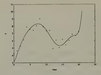
Figure 1:An eighth-order polynomial in time fitted to 21 observations on a random walk.

Figure 2:A first-order polynomial in time fitted to 21 observations on a random walk.
Parameterizing vector autoregressions
The autoregressive representation has too many parameters to be useful for applications to the short data sets that economists work with. It imposes little more than that are well defined, i.e. that the process is covariance stationary. In terms of describing a data-generating mechanism, the representation affords no economies in terms of numbers of parameters vis-à-vis either the entire list of covariance matrices or, equivalently, the spectral density . (Even though it provides no economies in terms of representation, the vector autoregression might provide insights.)
Applying vector autoregressions requires adopting special versions in which the numbers of parameters are kept small relative to the length of the data sets being studied. Economists have devised differing specializations designed to render the vector autoregressive model applicable.
Rational expectations macroeconomists and econometricians have devised one set of procedures for reducing the number of parameters. In addition to restricting the lag-length (instead of fitting an infinite-order vector autoregression, they fit models in which depends on only lagged values of itself), they typically restrict the number of coefficients that describe the cross-variable dynamics. They use theories that imply a particular class of functions expressing each coefficient matrix in the vector autoregression as a function of a much smaller number of free parameters . These parameters are interpreted as describing the preferences, technologies, and information sets of the agents whose behavior is determining . Such rational expectations models typically claim to be complete and fully interpreted models in the sense that they purport to describe the covariation through time of all of the variables modelled in ways consistent with general equilibrium theory, with the parameters being economically interpretable as preference, technology, or information parameters.[13]
Sims, Litterman, and their co-workers have invented a different way of coping with the overfitting problem. In principle, their procedures do not restrict the number of parameters (beyond their use of some restrictions on lag lengths), but work by heavily exploiting some of the computational features associated with a recursive form of estimation that is applicable to vector autoregressions. Rather than adopting a function as the rational expectations modellers do, Sims and Litterman carry along all of the elements of the ’s as free parameters, but restrict the initial coefficients and covariance matrix. Then they update all of the coefficients via recursive least squares. Evidently, their estimation procedures (or sometimes important parts of them) have interpretations as stochastic approximation algorithms.[14] Litterman and Sims have devoted much effort to devising specifications of these initial conditions that are designed to forecast macroeconomic time series well out of the sample used to estimate the parameters. Litterman and Sims’s choice of these initial conditions has involved less formal use of economic theory than that used by rational expectations econometricians in deducing their functions .[15]
Statistics for bounded rationality
The boundedly rational agents that we shall put into our example economic environments will all use versions of the stochastic approximation algorithm to estimate decision functions or parameters. This strategy for modelling boundedly rational agents starts from the observation that first-order conditions for stochastic estimation and optimization take exactly the form of the equation being solved by stochastic approximation, namely,
Further, stochastic approximation is designed to solve this equation under the conditions of limited knowledge (i.e., insufficient knowledge to use the differential calculus or the expectational calculus) with which we want to endow our artificially intelligent agents.
We shall see stochastic approximation algorithms applied over and over again, in superficially different contexts. Sometimes they will be used with versions of boundedly rational agents’ first-order conditions that come from estimation problems like those described in this chapter. Stochastic approximation algorithms will also be used where (9) is interpreted as the ‘Euler equation’ from a boundedly rational agent’s optimum problem.
Before handing stochastic approximation algorithms to our boundedly rational economic agents, we turn in the next chapter to survey some of the themes in the recent literature on neural networks and other forms of artificial intelligence. In reading this material, watch for stochastic approximation methods to make appearances.
A third aspect of data interpretation is the study of the quality of approximation, in which an analyst studies the behavior of some estimates that would be appropriate under the assumption that model A is correct when in truth model B has actually generated the data set. Sims (1972), White (1982), and Hansen and Sargent (1993) have studied the issue of approximation in various contexts.
Lennart Ljung (1977) and Ljung and Söderström (1983) have written extensively about the connection between stochastic approximation algorithms and some associated ordinary differential equations. Among economists, M. Aoki (1974) was one of the first to show the applicability of the stochastic approximation algorithm to study learning. See Ljung, Pflug, and Walk (1992) for a description of recent developments.
Prior information about the mean can be represented by using an initial condition other than 0.
For this estimator, the associated differential equation is , whose solution is , which converges to for any initial value .
Kuan and White (1991) show that the recursive estimators are root- consistent and share the asymptotic distribution of (non-recursive) nonlinear least squares.
In the estimation literature, ‘on-line’ algorithms refer to estimators that have the recursive structure of, for example, stochastic approximation algorithms, the estimator at being represented as a function of the estimator at and the data observed at . ‘Off-line’ estimators have the property that the estimator at cannot be expressed in this way; instead, the estimator at must be written as a function of the entire sample of observations up to time .
See Kendall (1957).
See Anderson (1958).
That is, for such data, the covariance matrix is ‘ill-conditioned’.
The method of Oja (1982) for grouping data amounts to a recursive implementation of principal components analysis.
See Sargent and Sims (1977) for remarks about the history of this interpretation of Burns and Mitchell (1946), and for details about how the static factor analysis model can be made dynamic via its application in the frequency domain in a way to encompass this interpretation of Burns and Mitchell.
Statisticians have dealt with the problem of overfitting by adopting criteria for choosing among parameterizations that penalize models with more parameters. The Schwarz Information Criterion (Schwarz 1978) is one widely used criterion; others are described by Rissanen (1989). Chung-Ming Kuan and Tung Liu (1991) apply and discuss some of these criteria in selecting among univariate models that are designed to predict future exchange rates. They report the results of employing the ‘Predictive Stochastic Complexity’ criterion of Rissanen. This criterion works as follows. Given a function designed to ‘forecast’ , and given a sample of length observations, compute the mean square of so-called honest prediction errors, namely, , where is estimated using data only through time . The model with the smallest value is the one selected by this criterion. Kuan and Liu find that it is difficult to pin down systematic nonlinearities that can be used to predict exchange rates better than by using a random walk theory of exchange rates.
Work along the lines of Hansen and Sargent (1980, 1981) and Kydland and Prescott (1982) fits within this category.
Doan, Litterman, and Sims (1984) describe a set of procedures for searching over some parameters (or hyperparameters) that pin down the initial conditions of the least squares recursions.
Sargent and Sims (1977) and Litterman and Sargent experimented with a factor analytic method for restricting the dimensionality of the parameter space for vector autoregressions. They used the frequency domain version of the factor analysis model, which assumes that the spectral density matrix of can be written , where is a matrix of rank for each , and is a diagonal matrix. This is equivalent to assuming that has the time domain representation , where is an vector process, each component of which is orthogonal at all leads and lags to each component of the vector of hidden factors . Sargent and Sims (1977) and Litterman, Quah, and Sargent (1984) used this model with to represent and evaluate Burns and Mitchell’s ideas about the business ‘reference cycle.’