4 Networks and Artificial Intelligence
This chapter describes some artificial devices that display ‘intelligence.’ Some of them memorize and recall patterns. Others represent and learn nonlinear decision rules. Most of the devices come from the recent ‘connectionist’ literature on neural networks. As Halbert White has taught, a student of econometrics will recognize many parallels between the connectionist literature and his own, in terms of problems and methods. The connections between the literatures on neural networks and econometrics provide additional perspective on our characterization of bounded rationality as a program to populate models with devices that mimic econometricians.[1]
The perceptron
The simplest neural network is a single-layer perceptron, a model of the interaction of input neurons , , with one output neuron . The neurons are elements and , where the spaces can be specified in various ways. For example, for ‘Ising neurons,’ ; for classification perceptrons we take . The perceptron model is
or
where and are each vectors, and is a ‘squasher’ function, i.e. a monotonically nondecreasing function that maps onto . Three popular squasher functions are:
The Heaviside step function:
The ‘sigmoid function’:
Any cumulative distribution function, e.g. the normal c.d.f.:
A perceptron is depicted graphically in Figure 1. Input is weighted by , inputs are summed across , then the sum is squashed to yield output . With the Heaviside squasher function, the neuron is either ‘on’ () or ‘off’ (). For non-negative inputs, a positive weight from input to the neuron is called an ‘exciting’ connection, and a negative weight is called an ‘inhibiting’ connection, because such connections make it more or less likely that the neuron will ‘fire.’
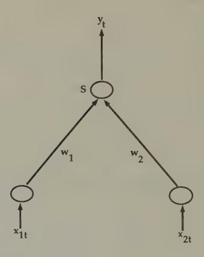
Figure 1:A perceptron. Values of two inputs for are multiplied by ; the results are added together, then operated upon with the ‘squasher’ function to produce the output .
The perceptron as classifier
For a given set of weights , a perceptron acts as a classifier. For example, let there be two classes of people, American football players () and economists (). Let be a vector of characteristics, say weight and salary, of individual .[2] When we present the perceptron with for economist , we want the perceptron to eject output , and when we input the characteristics of a football player, we want the perceptron to say . With the Heaviside step function as the squasher, the neuron ‘fires’ () if and only if . With one of the other two squasher functions above, the value of could be interpreted as the probability that an individual is a football player.
Perceptron training
Suppose that we have observations on characteristics of two distinct predetermined populations, again say economists, whom we have labelled , and football players, whom we have labelled . We want to fit the perceptron to these data, which means that we want to estimate the weight vector . We have a ‘training sample’ , where denotes a particular individual. The perceptron training problem is to choose to minimize . This is a nonlinear least squares problem. The literature on perceptrons describes various algorithms of the iterative form
where is a nonincreasing sequence of positive numbers, and is the gradient of with respect to . One scheme is to pick equal to a small positive constant, and repeatedly to run the sample through the algorithm until convergence occurs. Implementations of nonlinear least squares found in the econometrics literature also apply directly.
Perceptrons and discriminant analysis
There is evidently a close connection between a perceptron and a simple linear discriminant function. Early work on the perceptron focused on determining which classes of objects could and could not be separated by a perceptron, with negative early results by Minsky and Papert (1969) contributing to a long period of disenchantment. Minsky and Papert’s negative judgement about the perceptron was based on its inability to represent a nonlinear discriminant function. Enthusiasm for perceptrons revived in the early 1980s when it was recognized that networks of perceptrons could approximate any nonlinear discriminant function.[3]
Feedforward neural networks with hidden units
The perceptron is the building block out of which many types of neural networks are constructed. By arranging banks of perceptrons into rows and linking elements of successive rows via weighted summation operators, we construct a feedforward neural network. Halbert White and various co-workers[4] have shown that feedforward neural networks are best regarded as approximators of nonlinear functions mapping vectors into vectors .
A feedforward neural network with one hidden layer is described by the two equations
The second equation describes the output of hidden unit , which is simply a perceptron. The first equation generates the output of the network by taking an affine function of the vector of outputs of the hidden units. The parameters of the network are the weights and . The network can be represented compactly as
An example of such a network is depicted in Figure 2.
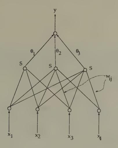
Figure 2:A feedforward neural network. The network takes inputs , multiplies them with weights and adds over to get the input into the hidden node , operates on the input into each hidden node with the ‘squasher’ function , then multiplies with and adds to get the output .
The literature has addressed two issues about models of this class: the issue of approximation or representation, and the issue of estimation. The approximation literature describes the class of functions that can be arbitrarily well approximated by model (8). Hornik, Stinchcombe, and White (1989) have shown that a very wide class of functions can be approximated by (8).[5] The parameter that controls the quality of approximation is , the number of hidden units. For a given , the best mean-square approximator to a function is determined by the values of that minimize the squared norm
Here is the norm. For a given , the best approximator can be found by variations on Newton’s method. The approximation literature comforts us by assuring us that, if we select large enough, we can find a that make this mean squared error as small as we might want.
The estimation problem occurs when we are given a sample and a particular model of the form (8), with fixed , and want to estimate the parameters. This is a version of the nonlinear regression problem. The model to be estimated can be written in the form
where we have stacked the parameters into the vector . Estimation can proceed by utilizing one of the algorithms based on equations (26) or (27) of the previous chapter. The ‘training’ algorithms discussed in the literature all use versions of these iterations. There exist examples of such ‘on-line’ algorithms that have asymptotic properties equivalent to ‘off-line’ algorithms. However, for small samples one can generally do better by using an ‘off-line’ algorithm.
Recurrent networks
The second equation of (7) can be modified in a way that lets us model dynamics. For example, we can specify
where is the vector of values of , and is a vector of additional parameters. This kind of network has been used by Elman (1988), and captures feedback to the hidden units from past values of hidden units. Alternatively, we could also specify
where is a vector of parameters. In the special case that for all , this is an autonomous dynamic system, one that can be used to represent the systematic part of a nonlinear vector autoregression; this specification is a version of a Hopfield network, to which we now turn.
Associative memory
This section describes a class of networks that store memorized patterns and solve some signal extraction problems. The simplest version of such a network is a dynamic system that has locally stable rest points at a predetermined number of memorized patterns. The network is designed so that, when a corrupted version of one of these patterns is injected, the network quickly converges to the closest memorized pattern.[6]
Autoassociation
Suppose that patterns are represented as vectors of length written in the binary alphabet , so that a particular pattern is expressed as a vector of 1’s and -1’s of length . There are patterns that we want memorized. Let these patterns be represented by the vectors , which we arrange into the matrix . We assume that the patterns are orthogonal, by which we mean that where is the identity matrix. It is assumed that is small relative to . The patterns correspond to ‘Platonic ideals.’
When the system is presented with an error-ridden signal in the form of a vector of length with elements , we want to know which pattern is the closest to the signal, as measured by the distance
That is, we want to know the value of for which the distance given by (13) is smallest. One procedure is simply to compute for each value of , and then select the one yielding the lowest value of . For large values of , this can be a time consuming process.
The idea of associative memory systems is to create a dynamic system
with the following two properties:
(a) Every memorized pattern is a fixed point of :
(b) Every is locally stable. That is, around each , there is a neighborhood such that, for , iterations on starting from converge to .
If such a dynamic system can be crafted, ‘recalling from memory’ is just the process of iterating on starting from a presented pattern. We want the convergence to occur rapidly.
Figure 3 portrays a ‘phase diagram’ of a Hopfield network with four memorized patterns. The arrows in the diagram indicate how the network is locally stable about each of the memorized patterns.[7]
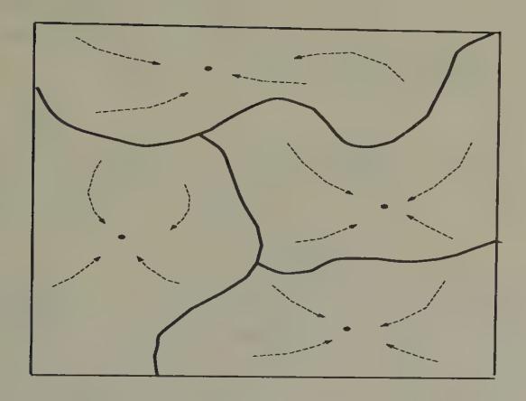
Figure 3:A Hopfield network. The network has four ‘memorized patterns’ that are attractors for the net’s dynamics.
It is easy to create a mapping with the desired properties. We use the Hopfield network
where is an matrix and sgn is the ‘sign’ function that maps real-valued vectors into vectors of binary numbers, mapping positive components into +1, negative components into -1. A common way to choose is according to Hebb’s rule:
It is straightforward to show that Hebb’s rule builds in properties (a) and (b). To verify property (a), let us input into the network the th pattern, , where . We want to be output, which we have because
Here is the unit vector with 1 in the th position, 0’s in all other positions.[8]
To study property (b), suppose that we input a noise-corrupted version of pattern , , where agrees with except for sign reversals at randomly selected positions. We set the dynamic system in motion starting from , and compute
where . The terms can be expected to be small because the pattern matrix is orthogonal, so long as the number of corrupted bits is small. Thus we have
The terms can be expected to have value on the order of , so that, as long as and , we have that
indicating that convergence to the desired pattern occurs in one step.[9]
Correlated patterns
It is easy to modify Hebb’s rule to accommodate correlated (but linearly independent) patterns. We now drop our earlier assumption that , and replace it by the assumption that
where is a nonsingular matrix. We maintain system (16), but replace Hebb’s rule (17) with the so-called ‘projection rule’:
It is easy to check that with this modified rule the rest points of are , as described, and that the system is locally stable about these rest points. To check the existence of as a fixed point, note that .
Heteroassociation
Hopfield networks can be ‘wired’ to remember sequences of patterns. Let represent a temporal ordering of patterns. When (or a corrupted version of it) is ‘input’ into the network, we want the ‘output’ from the network to be , where we understand that , so that the memorized pattern is to be periodic. This is easily achieved by using a modified version of Hebb’s rule. Let , , . Let
Note that the system
has the periodic solution , for we have
where again is the unit vector with one in the th place.
Memorized patterns as energy minimizers
Associated with Hebb’s rule (17) is the energy function[10]
By construction, the stored patterns are each local minimizers of this function. In particular, note that
for , , and that, since for all , we know that is a local minimizer. For the ‘projection rule’ , we have the associated energy function
Stochastic networks
Sometimes Hopfield networks are constructed that have spurious local rest points that the designer wants to avoid. When these rest points have small domains of attraction, they can be avoided by using a stochastic network. The idea is to modify the dynamics of the system by ‘shaking’ it at a rate that decreases over time. The purpose of shaking the system is to lower the probability that the system will come to rest at ‘undesirable’ local rest points and descend to better ones. Figure 4 and Figure 5 contain an example of what is hoped for. Introducing a random ‘shaking’ factor into Newton methods leads to what are called ‘simulated annealing’ methods.[11]
The dynamics of a network with neurons , , can be represented
where is one of our ‘squasher functions.’ For example, we might use
as a squasher function for ‘Ising neurons’ that we want to constrain to take on values in .[12] The variable is a ‘temperature’ variable that governs the sharpness of the squasher function.
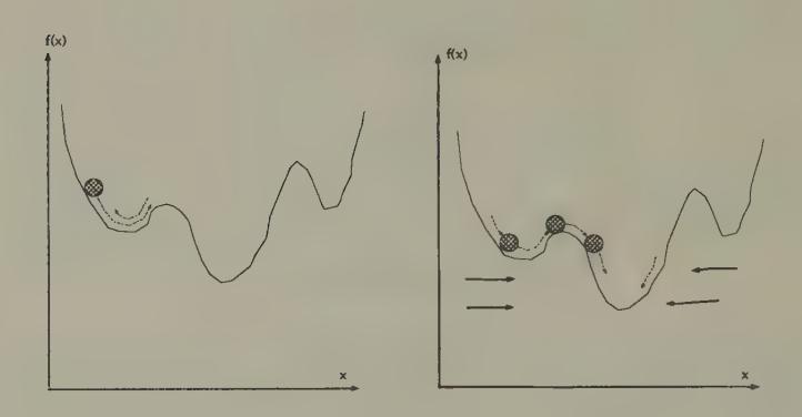
Figure 4:Newton’s method. Motion of a ball rolling down a hill under force of gravity. The ball may come to rest at a local minimum.

Figure 5:A stochastic Newton method. Simulated annealing and ‘stochastic network’ methods ‘shake’ the system so that with probability arbitrarily close to one the ball will eventually escape being trapped in a local minimum.
Combinatorial optimization problems
Neural nets have been used to solve constrained optimization problems that can be represented in the form: find a configuration of neurons , , to minimize
where is a given matrix encoding costs, and is a penalty variable (or Lagrange multiplier). One approach to this problem would be to use the deterministic ‘local dynamics,’ i.e. those given by the Hopfield network,
However, this algorithm typically fails to find a global minimum, and instead heads for the nearest local minimum.[13]
To get an algorithm with a better chance of descending to a global minimum, the deterministic local dynamics are sometimes replaced by stochastic ones. Let be the probability that is plus or minus 1. Then we can generate stochastic dynamics by setting
where is a non-negative temperature variable. This stochastic transition law produces a stochastic process with a stationary distribution over states given by the Boltzmann distribution
where the normalization factor is
As approaches zero from above, this distribution concentrates more and more probability on the global minimum of the cost function (32).
The method of simulated annealing exploits this property. The algorithm works as follows. For a fixed initial and a given initial configuration of neuron values , use the stochastic dynamics, say via simulation methods, to compute a sample from the stationary distribution for that fixed . This represents a sample drawn from the Boltzmann distribution (35). Now define an iterative process in which the system is ‘annealed’; i.e., the temperature is gradually lowered, at a rate slow enough to permit the system approximately to settle into its stationary distribution at each temperature. In particular, lower the temperature, say according to , where is the temperature at the th step; use the (approximate) stationary distribution from temperature as an initial distribution; and use the transition dynamics at this new temperature to get an estimate of the probability distribution (35) associated with this new temperature. Continue in this way, lowering the temperature toward zero. Notice that as approaches zero the probability given by (35) piles up near optimizing values of the state vector .
This procedure is computationally intensive, but has the virtue of assuring convergence to a global minimum of the cost function. The computational expense occurs at the step of computing the stationary distributions (35) at each temperature.
Mean field theory
The idea of mean field is to replace the stochastic dynamics with an associated deterministic dynamics that gives the correct direction of movement ‘on average.’ The basic object of analysis is the time average of neuron at temperature , which we denote or for short. The variable is the average value of neuron in the stationary equilibrium given by (35). The approximate mean field dynamics are given by[14]
Equation (37) is a set of deterministic difference equations in the average states of the neurons. Notice the similarity between systems (30) and (37).
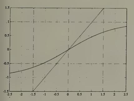
Figure 6:The function with . Fixed points are at intersections with the dotted line of slope 1 through the origin.
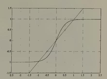
Figure 7:The function with . Fixed points are at intersections with the dotted line of slope 1 through the origin. At lower temperatures, the fixed point at 0 becomes unstable, and two stable fixed points near appear.
The dynamics of the system (37) are known to exhibit behavior of two sorts, depending on the temperature . At sufficiently high temperatures, the system moves to a steady state at , which can be seen to be the fixed point of the tanh function (see Figure 6 and Figure 7). As the temperature is gradually lowered, a ‘phase transition’ is passed at a critical temperature , and the system moves to fixed points that approximate a solution of the minimization problem. Peterson and Söderberg describe methods for estimating the critical temperature . These methods start from a Taylor series approximation of (37) around , which yields the dynamics
where . The stability of the local dynamics around are determined by the eigenvalue of maximum modulus of the matrix
For large enough, the dynamics around are evidently stable. However, for nontrivial , there will exist a critical value at which an eigenvalue of will exceed unity in modulus, causing the linear dynamics to destabilize and prompting the nonlinear aspects of the dynamics of system (37) to take over. Peterson and Söderberg describe computationally efficient methods for estimating the value of from the pair . They also describe corresponding methods for similar but richer problems.[15]
Here is Peterson and Söderberg’s implementation of mean field dynamics to minimize a cost function of the form (32).
(a) Compute an estimate of the critical temperature . Set , or for , where is to index iterations.
(b) Initialize the (mean-field) neurons randomly to values .
(c) For , iterate on the mean field dynamics (37).
(d) Reset temperature according to, e.g., and repeat step (c). Continue to iterate until the criterion function ‘settles down.’
Peterson and Söderberg (1992) provide several examples in which the mean field dynamics provide cheap and high-quality approximate solutions to some big optimization problems.
Shadows of things to come
Mean field theory uses a deterministic system whose dynamics approximate aspects of the average behavior of a random dynamical system. The deterministic system is formed by writing down the random dynamical system, then replacing random variables with their means at carefully chosen spots. This procedure has provided a cheap way of solving or approximately solving some high-dimension combinatorial optimization problems.
We shall encounter this kind of device again, in different contexts. In particular, we shall see how closely related arguments from the ‘stochastic approximation’ literature have been applied to study the convergence of systems of boundedly rational agents to rational expectations equilibria.
Local and global methods
Newton’s method, which is the basis for many of the estimation methods that we have surveyed, has excellent local convergence properties, but can have difficulties globally. Simulated annealing and stochastic Newton methods are modifications designed to improve the global properties of Newton’s method without eventually sacrificing its good local properties. We now turn to some global search algorithms proposed by Holland that depart more fundamentally from Newton’s method.
The genetic algorithm
The genetic algorithm of John Holland was devised to find maxima of ‘rugged landscapes’ that lack the smoothness that Newton’s method exploits.[16] Holland’s idea was to turn loose on the landscape a population of sexually active artificial beings that would evolve itself to the top of the hill.
The genetic algorithm is a sequence of operations applied to a population of binary strings, which are strings of 0’s and 1’s of length . Recall that each integer in the collection can be represented as where is the value (0 or 1) in the th position in the string. We can approximate a bounded set of real numbers by setting , where are chosen to select the set that we want to approximate.
The algorithm begins with a collection of binary strings of length . We are given a non-negative function , which we are to maximize. We encode values of , where may be a vector space, in terms of binary bit strings. We are told how to compute for any value of within the domain defined by our encoding.
The algorithm uses the following operators.
Evaluation of fitness. For every value for , compute the value . Then compute the ‘relative fitness’ of , defined to be .
Fitness-proportional reproduction. Make copies of the population by spinning a ‘biased roulette wheel,’ constructed by dividing a disk into slices, with the probability of individual ’s reproducing being set equal to its relative fitness . Spin the wheel times, each time making a copy of the individual into whose slice the roulette ball comes to rest, thus making copies. The copies constitute a new population of individuals.
Mutation. Independently subject each bit of each string to a small probability of being flipped.
Mating. Randomly divide the population of strings into equal subpopulations of ‘males’ and ‘females.’ Randomly match these subpopulations into pairs for the purpose of ‘mating.’ A pair (sometimes referred to in the literature as ‘the happy couple’) mates by drawing a random number that is uniformly distributed across the integers from 1 to . If the integer is drawn, the male’s and female’s bit strings are each cut between the bit numbers and , and two new strings are formed by joining the first bits of the male string with the last bits of the female string, and vice versa. In this way are formed ‘children’ strings. Extinguish the parents, and take the children as the new population.
The algorithm starts by selecting a random sample of strings, and then applying the four operators sequentially. After a new population is created via the mating operator, the algorithm applies operator 1 again, continuing either for a prespecified number of rounds or else until a stable population of ’s emerges. As the ‘solution’ of the original problem, select the fittest member from the final population. The parameters of the algorithm are , , and the mutation rate .
The reproduction operator increases the representation of relatively fit individuals in the population, but does nothing to find a fitter individual. The mutation and mating operators can add new elements to the population, while destroying old ones. If the mutation probability is set too high, it slows or prevents convergence, and degrades the performance of the algorithm because it destroys fit individuals along with the unfit. But when the mutation rate is set to a very low value, mutation alone is a poor mechanism for injecting diversity into the population. The mating operator seems to be a very good device for probabilistically injecting diversity, while giving structures that have proved their fitness a shot at surviving.
This algorithm has proved its value in a variety of applications. It has some features of a parallel algorithm, both in the obvious sense that it simultaneously processes a sample distribution of elements, and in the subtler sense that, instead of processing individuals, it is really processing equivalence classes of individuals. These equivalence classes, which Holland calls schemata, are defined by the lengths of common segments of bit strings. The algorithm is evidently a random search algorithm, one that does not confine its searches locally. The mating operator, which lies at the heart of the algorithm, creates new strings, but only when it operates on a population within which there is already diversity. The beauty of this operator is that, while it creates new values of (at the cost of destroying old ones), it does so in a way that preserves long sections of ‘genetic structure,’ i.e. segments of bit strings. Depending precisely on how a given problem has been encoded, this feature can embody a useful compromise between the principles of adventure and preservation.
The genetic algorithm is designed to produce a sequence of populations of organisms that moves up a fitness criterion . The ‘individuals,’ i.e. the bit strings, do not ‘learn.’ (Each of them dies after one period.) Only the ‘society’ of the sequence of populations of bit strings can be regarded as learning. This feature makes it difficult to accept the genetic algorithm literally as a model of an individual ‘brain.’ It is much easier to relate to John Holland’s classifier system as a model of an individual’s brain or thought process.[17]
Classifier systems
The brain as a ‘competitive economy’
John Holland conceived the ‘classifier system’ as an evolving collection of potential ‘condition–action’ statements that decide and learn. He used an alphabet for expressing the rules that permits more general statements to co-exist with less general statements. The statements compete with one another for the opportunity to decide. The classifier system incorporates elements of the genetic algorithm with other aspects in a way that represents a brain in terms that Holland describes as a competitive economy.
A classifier system consists of a more or less comprehensive list of ‘if-then’ statements called classifiers that map conditions into actions, and a set of rules for interpreting and altering these statements to make decisions through time. A classifier system has a list with a fixed number of classifiers. When a message from the environment enters the classifier system, in general, several of the classifiers will have their ‘if’ parts satisfied, but usually their ‘then’ parts will differ, in which case these classifiers are offering different advice (‘Go on, say hello to her’ versus ‘Mind your own business’). Which classifier makes the decision is determined by an ‘auction’ among the relevant set of classifiers, with classifiers bidding with ‘resources’ accumulated via an accounting process that registers the consequences of past decisions. The accounting system is the vehicle by which the classifier system learns to alter its behavior over time.
More formally, a classifier system consists of the following objects.
Bit strings (classifiers). A classifier is a bit string of fixed length, written over the trinary alphabet , where is interpreted as ‘either 0 or 1’ or ‘I don’t care.’ The first part of each bit string is interpreted as encoding a ‘condition’ statement, while the remaining bits encode an ‘action’ statement. The presence of the sign accommodates generalization.
A decoding device. When a state occurs in the environment, this device identifies which of a fixed collection of classifiers match in their ‘condition’ parts the condition prevailing in the environment. The device thereby identifies a set of classifiers, from which one is to be selected actually to make a decision at the moment.
An accounting system. A measure of value called strength is assigned to each classifier in the system at each point in time. Strengths for each classifier are updated over time in response to the utilities and costs that flow from the environment when the classifier acts. The accounting system computes cumulated averages of realized utilities net of costs. In sequential settings, the accounting system taxes classifiers operating at one stage, and awards the proceeds to the classifier at the immediately preceding stage of the decision tree whose decision moved the system to the position that gave the presently active classifier the opportunity to act. Setting up the accounting system in this way is important to induce decisions whose only rewards are that they facilitate subsequent decisions that will ultimately generate rewards.
An auction system. The auction system determines which of a set of matched classifiers is granted the right to act in any given situation. Two alternative auction principles are:
(a) The highest strength rule gets to make the decision.
(b) The right to make a decision is allocated probabilistically, with the probability of being granted the decision made equal to a rule’s relative strength.
A device for introducing new classifiers. New classifiers are introduced in several situations.
(a) Uncovered situations. The most obvious occurs when the environment produces a condition that matches no existing classifiers. In this situation, a new classifier is generated whose condition statement matches the existing environmental condition, and whose action part is randomly generated.
(b) Try something new. New classifiers are generated and old ones are occasionally extinguished in order to provide room for experimenting with untried actions.
(c) Generalize and specialize. New classifiers are synthesized to generalize (replace 0’s and 1’s with 's), or to specialize (replace 's with 0’s or 1’s in existing rules).
A two-armed bandit
An example of Brian Arthur and Carl P. Simon illustrates a method for studying the limiting behavior of a classifier system in a very simple context. In particular, they showed how a classifier system would cope with a two-armed bandit problem.[18] The th arm pays a random variable drawn independently and identically from a distribution with mean . Assume that . A player must pull one arm for each with , with his reward being his total payoffs. The player knows neither nor .
Arthur let the classifier system consist of the two classifiers,
#0
#1
Here the first entry encodes the ‘condition’ and the second entry encodes the ‘action’; means ‘whatever the history of observations,’ 1 means pull the first arm, and 0 means pull the second arm. The conditions of both classifiers are met all of the time. The first classifier plays arm 1 all of the time, and the second plays arm 2 all of the time. Let , , be a clock recording the cumulative number of times that arm has been pulled as of time , which equals the cumulative number of times that classifier has acted. Arthur set up the accounting system
where is the ‘strength’ of classifier after it has been rewarded with its payoff when its clock is at .
Arthur used a random device based on relative strengths to determine the advice of which classifier was followed at time . In particular, at time , the system follows the advice of classifier 1 with probability given by
By using methods of stochastic approximation, Arthur showed that the classifier system eventually ‘probability-matches,’ that is, plays the arms in fractions-over-time that are in proportion to their expected rewards.[19]
Design decisions
An author of a classifier system controls the list of states or conditions to encode, the scheme for encoding them, and the accounting system that distributes rewards and collects ‘taxes.’[20] Thus, some ‘hard wiring’ goes into the construction of a classifier system, much of it being done with an eye to the particular problem at hand. In some environments, what is not hard-wired is the degree of generalization.
Generality versus discrimination
The problem of learning induces an incompletely understood tradeoff between ‘general’ rules (those with ‘conditions’ that are coarse and therefore are often met) and ‘specific’ rules (those with conditions that are fine and therefore less frequently met). An advantage of ‘general’ rules is that their conditions are frequently encountered, which means that their performance can be assessed frequently. A disadvantage is that they call for the same action for all states that satisfy the condition. In effect, general classifiers give the advice: ‘use a piece-wise constant decision rule over the subset of the state space that I cover.’ Specific decision rules have the opposite advantages and disadvantages. They potentially permit fine-tuning the action to fit the specific point in the condition space, but they pay for that advantage by requiring longer histories of experience to learn.[21]
An interesting property of classifier systems is that they can be set up in ways that permit the degree of generalization or specificity to emerge adaptively. The presence of the (or ‘I don’t care’) symbol in the alphabet, together with devices designed either to generalize or specialize,[22] provide this capacity. The literature has some intriguing simulation examples in which different degrees of generalization have emerged in classifier systems, but at the present time little is known about general principles that determine their propensity to generalize.
Summary
In this chapter we have seen recursive least squares dynamics appear in many guises and contexts. There are evidently many fascinating connections between research lines being pursued within the ‘connectionist’ literatures that we have surveyed in this chapter and the econometrics and statistics literatures described in the preceding chapter. It is tempting (and would surely be worthwhile) to pursue those connections more broadly and deeply, but it is time for us to redirect our attention to our main task of discussing economic models of bounded rationality. In the next chapter we hand over some recursive least squares algorithms to artificial agents living within one of several particular economic environments, and watch what happens.
Useful references on some of the material in this chapter are Müller and Reinhardt (1990), Hertz, Krogh, and Palmer (1991), and Kosko (1992).
Most American football players are heavier than the average person. Some economists are also heavier than the average person.
In-Koo Cho (1992) shows that a pair of single-layer perceptrons can represent all subgame-perfect strategy pairs in an infinitely repeated (undiscounted) prisoners’ dilemma game. A key part of his demonstration is that a single-layer perceptron is ‘discriminating enough’ for the situation each player confronts. Cho shrewdly exploits the ease with which a perceptron can implement a ‘trigger strategy’ via a squasher function. For another infinitely repeated two-player game, Cho shows that a single-layer perceptron is too simple (because it is unable to discriminate among situations adequately), but that a network with one hidden layer is able to encode all subgame-perfect equilibrium strategies.
Including Ronald Gallant, Kurt Hornik, and Maxwell Stinchcombe.
They show that, if enough hidden units are included, then any Borel measurable function from one finite dimensional space to another can be approximated arbitrarily well. Barron (1991) showed that to achieve the same approximation rate a feedforward network uses only linearly many parameters (), while polynomial, spline, and trigonometric expansions use parameters that grow exponentially ().
Hertz, Krogh, and Palmer (1991) and Müller and Reinhardt (1990) are good references on the material in this section. Müller and Reinhardt provide an example in which a Hopfield network is used to ‘read’ noise corrupted letters encoded in pixels via ‘Ising neurons.’
A problem in constructing associative memory models is that sometimes the builder inadvertently puts ‘spurious patterns’ into the network, so that the network recalls patterns that weren’t taught to it. Notice that the construction in the text assures that the ‘memorized patterns’ are rest points of the network, but does not preclude the presence of other rest points.
Notice that because .
There is a literature on ‘response times’ in cognitive psychology in which subjects are asked to classify a specific example (‘pelican’) into one of a specified number of classes (‘central banker,’ ‘bird,’ ‘congressperson’). Their times to respond are recorded and interpreted in terms of the closeness of the particular item to the ideal pattern. The Hopfield network is a useful device for interpreting these experiments.
If the formulas associated with Hebb’s rule remind the economics student of things from econometrics, they should.
This section relies heavily on Peterson and Söderberg (1992).
Or , if we want the neurons to take values in .
This local stability property is ‘good’ for models of associative memory, but ‘bad’ for schemes that iterate on first-order conditions from optimum problems.
See Brock (1992) for several applications of mean field dynamics to models of economics and finance.
Goldberg (1989) is a useful text on genetic algorithms.
Ellen McGrattan has applied genetic algorithms to estimate nonlinear rational expectations models. She first uses genetic algorithms to search for the vicinity of a maximum, then switches to a Newton method.
These results were presented by Arthur (1989b) and Simon in independent oral presentations at the Santa Fe Institute in March 1989.
See Arthur (1989b) for discussions of various ways of altering the classifier system to improve its performance.
In sequential problems, the author must also link classifier sub-systems ‘intertemporally’ in ways that permit learning to experience the rewards of patience. See Marimon, McGrattan, and Sargent (1990) for an example.
This might remind the reader of tradeoffs between parametric and non-parametric estimation strategies in econometrics.
See Marimon, McGrattan, and Sargent (1990).