Adaptation in Artificial Economies
This chapter puts adaptive agents into five different environments that have been analyzed in the rational expectations literature, thereby illustrating some of the different structures and possibilities in economic systems composed of such agents.
The first model, due to Bray, nicely illustrates many features of ‘least squares learning’ in a ‘self-referential’ system, including the temporary irrationality of adaptive forecasting rules and the possibility of their eventual rationality. The second model, a version of Samuelson’s overlapping-generations model of money, illustrates how successive generations can adaptively climb their way to more or less complicated rational expectations equilibria, and how the rate of convergence can depend on details of the adaptation algorithm and the intricacy of what must be learned. The third example puts overlapping generations of adaptive agents into an environment with too many equilibria, namely, a multiple currency setting in which the substitution of adaptive for ‘rational’ agents is enough to render the exchange rate determinate, but history dependent. The fourth example is a version of the ‘no-trade’ environment of Jean Tirole, in which the ‘problem’ with the rational expectations equilibrium is its incredible efficiency in eliminating opportunities for trade based on disparate information; I show how replacing rational agents with adapting ones can serve temporarily to restore opportunities for trade and thereby create trading volume. The last example, Marcet and Sargent’s model of investment under uncertainty with learning, is designed to illustrate how much ‘coaxing’ must be done by us and how much ‘theorizing’ must be done by our artificial agents for them to learn when their planning horizon is infinite.
The presentation in this chapter is informal. We spend most of our effort describing and simulating models. The chapter is concluded with a brief description of how the machinery of stochastic approximation can be used to attain analytical results about the limiting behavior of such models.
A model of Bray
Margaret Bray (1982) studied a model that exhibits several features of systems that are adapting their way to a rational expectations equilibrium. These features include:
(a) People use a forecasting scheme that would be optimal if the environment were stationary. But their learning causes the environment to be non-stationary, and their learning scheme suboptimal.
(b) Sometimes the system converges to a rational expectations equilibrium.
(c) If the system does not converge to a rational expectations equilibrium, it does not converge.
(d) The dimension of the ‘state’ of the system with learning is larger than the corresponding rational expectations equilibrium, because measures of people’s beliefs are needed to describe the position and motion of the system.
In Bray’s model, the environment would be stationary if people were to know the distribution of prices. The dynamics in the model all come from the adjustment of people’s expectations, which vanish if and when people learn the equilibrium distribution of prices.
Bray assumed a ‘cobweb’-like structure in which the equilibrium price for a single commodity is determined by a market-clearing condition of the form
where is the price that market participants expect to prevail at time , and is an independently and identically distributed sequence of random variables with mean zero. To compute a rational expectations equilibrium, we note the absence of dynamics in either the structural equation (1) or the shock , and so we guess that , a constant that is independent of time. Substituting this guess into (1) gives , which implies . Evidently, the guess is true if . Substituting this value of back into (1) shows that in a rational expectations equilibrium .
In backing off rational expectations, Bray assumed that people form the expectation by taking an average of past prices. For convenience, we use the notation . In terms of a stochastic approximation algorithm, Bray’s assumption about expectations can be represented as
Notice how this scheme uses only observations on prices through period to form price expectations at time .
Rewrite equation (1) by substituting for to get
Given an initial condition for , equations (2) and (3) determine the evolution of through time, where is interpreted as people’s expectation of what will be.[1] Bray studied the circumstances under which and the distribution of , which evolve interdependently, would converge to a rational expectations equilibrium. That is, she studied the conditions under which would converge to the value .
For describing people’s learning behavior, we can use a state vector , whose law of motion is evidently
This system indicates that, when at time people estimate the price next period to be , they act to make the best prediction of next period’s price be . Notice that in forecasting this way people are acting as if they believe (incorrectly) that the law of motion of the state is not (4) but rather
for some serially uncorrelated random process with mean zero, where is a constant. When people perceive that the law of motion for is governed by (5), their forecasting causes the actual law of motion to be (4).
Margaret Bray showed that, if , system (2), (3) will converge to a rational expectations equilibrium with probability one. She also noted that is a necessary condition for convergence to a rational expectations equilibrium.[2] Furthermore, she showed that, if the system does not converge to a rational expectations equilibrium, it does not converge at all.[3]
Irrationality of expectations
Although the model’s exogenous ‘fundamentals,’ i.e. the process and the parameters , , are stationary, the stochastic process for the price is nonstationary, because it is a piece of the joint process determined by (2), (3). This means that the expectations formation scheme (2), which is a sensible way to estimate a mean for a stationary process (e.g., for someone already living within the rational expectations equilibrium of this market), is suboptimal so long as expectations are being revised. The fact that in (3) is moving through time, as described by the law of motion (4), means that is itself a ‘hidden state variable,’ and that the system (4) should be augmented to include it. Substituting (2) into (3) and rearranging gives the following system:
This is a nonlinear stochastic difference equation, which can be used to forecast prices with smaller mean squared error than given by the forecast used by the people in the model. In particular, the expectation of conditioned on the entire state is equal to
Equation (7) gives the ‘rational expectation’ of price conditional on the full state vector . This is the price that would be forecast by an outside observer who knew that the price was determined by (2), (3), and who could observe (or compute) as well as . The failure of this conditional expectation to equal , except after convergence, indicates the irrationality of the learning scheme.
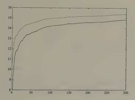
Figure 1:Simulation of (solid line) and the rational expectation (dotted line) in Bray’s model starting from . The variance of was set at one. The conditional expectation is the best forecast of price that could be made by an outside observer who understood that agents are learning via Bray’s scheme.
Figure 1 and Figure 2 display aspects of a simulation of Bray’s model in which we set , , . The random process was generated with a Gaussian pseudo-random number generator. The rational expectations price is . We started the system at , an expected price far below the rational expectations price. Figure 1 shows the gap between the least squares forecast and the conditional expectation , which is large at first, then gradually diminishes over time. Figure 2 and Figure 3 show how the rational expectations forecast on average is closer to the actual price than is .
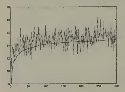
Figure 2:Simulation of (dotted line) and in Bray’s model. The forecast on average underpredicts , but the underprediction tends to diminish with time.
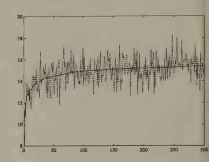
Figure 3:Simulation of (dotted line) and in Bray’s model.
Why not repair the irrationality indicated by the discrepancy between and by going back to the original model and replacing by ? Evidently, using this new theory of price expectations would require us to modify the actual law of motion for prices, which would render our new scheme suboptimal again. But we can use this new actual law of motion as our theory of expectations. This line starts us on a recursion, which has been taken up by Bray and Kreps (1987), who show that in the limit it leads us back to a rational expectations in which agents are learning ‘within’ the equilibrium, but not ‘about’ the equilibrium. Bray and Kreps argue against following this recursion to its limit if it is ‘bounded rationality’ that we are after.[4]
Heterogeneity of expectations and size of the state
Bray’s model assumes that all market participants have the same beliefs . If we permit heterogeneity of beliefs, the effect is to add to the dimension of the true state in the appropriate counterpart to (6). For example, suppose that there are two classes of agents, differentiated only by the initial , say and , which they use in a version of scheme (2), and that each of the two classes accounts for half of the market. Then the counterpart to (6) would include as state variables. In this version of Bray’s model, heterogeneity of beliefs would vanish as the system converges to a rational expectations equilibrium.[5]
An economy with Markov deficits
The second example is the overlapping-generations model of a monetary economy introduced by Paul Samuelson, and used extensively by John Bryant, Neil Wallace, and others to study issues of inflationary finance. We use this model to illustrate how:
(a) Learning can be modelled by having overlapping generations of agents adjust their behaviors relative to those of their ancestors in a utility increasing direction.
(b) The object about which agents are learning can be specified ‘non-parametrically,’ provided that agents are patient enough or lucky enough to be willing to learn how to behave on a state-by-state basis.
(c) Where the state is of high dimension, agents can be modelled as learning by using parametric decision rules.
(d) There is a close connection between algorithms to compute (approximate) equilibria and models of learning.
The economy consists of overlapping generations of two-period lived agents. At each date , there are born identical agents who are endowed with units of a single consumption good when young, and units when old. Each young agent’s preferences over a lifetime consumption profile are ordered by the expected value of , where , where .
There is a government that prints currency to finance government expenditures that are governed by a Markov chain
We let be the possible levels of government expenditures. The government’s budget constraint is
where is the stock of currency carried over by the young at to , and is the time price level.
Stationary rational expectations equilibrium
The rate of return on currency between and is . We shall seek a stationary equilibrium in which the rate of return on currency is given by
Finding a stationary equilibrium requires solving a set of nonlinear equations in a set of vectors characterizing individual agents’ optimal decisions. In a stationary equilibrium, savings are determined by an vector of state-dependent saving rates where and is the saving rate when .[6] A young agent’s utility is given by
for where is an increasing and concave utility function. The first-order conditions with respect to are or
In a stationary equilibrium, the government’s budget constraint, namely, , can be written as
where when .
Finally, the condition that the supply of currency must equal the demand can be written or
To determine a stationary equilibrium, we have to solve equations (12), (13), and (14) for vectors and and an matrix of rates of return, where the ’s satisfy and the elements of are all positive. Notice that (13) and (14) imply
Substituting (15) into (12) gives the following set of nonlinear equations to be solved for :
Evidently, a stationary equilibrium exists if and only if (16) can be solved for with for all .
In general, the system of nonlinear equations (16) that determines a vector of stationary equilibrium saving rates has multiple solutions. In addition to multiple stationary equilibria, there are nonstationary equilibria of the model, with a form resembling the ‘bubble equilibria’ of the models of money described in Chapter 2 and which we shall meet again in Chapter 6. Overlapping-generations models of the type we are using also have stationary ‘sunspot equilibria,’ that is, equilibria in which random variables (called ‘sunspots’ or ‘extrinsic random variables’) influence equilibrium prices and quantities only because they are expected to influence them.[7] The stability of sunspot equilibria under adaptive learning has been studied by Woodford (1990), Evans (1989), and Evans and Honkapohja (1992a).
A learning version
We use this environment as a setting in which successive generations of agents are ‘learning’ or ‘evolving.’ We want to watch how collections of adapting agents cope with the environment, and see whether and when they might eventually learn the rational expectations equilibrium. We can also watch how agents’ learning varies as we alter the complexity of what they learn about, which in this setting is controlled by the number of states and the stochastic structure of the Markov process for government expenditures.
We endow agents with knowledge about their own utility functions, about the previous experiences of agents like themselves, and about the behavior of past and present government expenditures and prices. However, we do not give agents knowledge of the distributions of government expenditures, prices, and rates of return. Instead of knowing these distributions, agents must somehow use their historical observations, which might be arranged in the form of histograms or empirical probability distributions, to make decisions by some principle other than that of ‘expected utility maximization with knowledge of equilibrium probability distributions.’
The economy with learning is identical with the model with rational agents, except that now the households consist of two classes (subsequences) of (adaptive) agents. We include two classes, called ‘odd’ and ‘even,’ because, in order to evaluate a person’s saving decision, we wait until two periods’ worth of consumption data for that person have become known. Odd agents reset a saving rate when is odd, while even agents reset a saving rate when is even. Odd agents learn from the past experiences of other odd agents, and even agents from the past experiences of other even agents. Agents of each class will be assumed to update their saving decisions based on the utility experienced by previous people of their type. In particular, they will adapt the decisions of their predecessors using a recursive Newton--Raphson (or stochastic approximation) procedure.[8] The ex post realized utility of a person who observed and set when young at time is
where is the realized gross rate of return. The derivatives of realized utility with respect to the saving decision are
Notice that, in a rational expectations equilibrium, , , where is the expectation conditional on . We want a learning algorithm to apply where people don’t know these conditional expectations.
We assume that people use a Robbins--Monro algorithm, state by state. To set up the Robbins--Monro algorithm, we have to keep track of the number of periods an individual has been in a given state (i.e., observed ) for each state. We let for index the cumulative number of odd and even generations, respectively. For each state , we let , , index the cumulative number of times that has equalled . That is,
We define the decreasing gain sequence . The learning algorithm is then
This algorithm is set up to promote the possibility that, as , we will have and will solve the first-order conditions .
We assume the one-period utility function . In the experiments reported below, we assume the logarithmic specification .
We assume that young agents observe before they make their saving decision. Agents of each type begin each period with an vector of saving rates , , ‘learned’ from ancestors of their own type, which they use as a state-contingent saving rule. When , the young at date set savings according to .
The price level at time is determined by the two equations
which imply
We require an initial condition for at , and initial conditions for for each of our two classes of agents.
We assume, as in the rational expectations version of the model, that is a Markov chain with transition matrix , where .
Some experiments
Figure 4 and Figure 5 report the results of using our learning algorithm. For each experiment, we set , and we set initial conditions for .[9] We studied two economies, identical in all respects except for the stochastic process for government expenditures. In each economy, government expenditures follow a two-state Markov process with transition matrix . In each economy, , for each type of agent. In the first economy, government expenditures are identically zero in both states and . This implies that the rational expectations savings rates are 5 for each ‘state’ of government expenditures, and that the equilibrium rate of return on currency is unity always. In the second economy, government expenditures follow a Markov process with
where the two states are . For the second economy, the equilibrium savings rates are , and the equilibrium rates of return are
For comparability, we model each of the economies as being driven by a two-state Markov process for government expenditures, though in the first economy this means that the agents are wastefully overfitting their saving function.
Figure 4 and Figure 5 indicate that both economies are converging to the rational expectations savings rate. The convergence occurs more and more smoothly as time passes, a feature caused by the action of the sequence.
Figure 4:Simulation of savings rates of odd agents for stochastic approximation algorithm when , , . The rational expectations equilibrium savings rates are 5 in each state. The saving rates (dark line for state 1, dotted line for state 2) are converging to the rational expectations saving rates.
In the zero expenditure economy, nothing stochastic is occurring. For this economy, convergence can be accelerated by using a constant-gain algorithm. This algorithm is formed by replacing the by a constant. Besides accelerating convergence in constant environments, a potential advantage of constant-gain learning schemes is that they retain their flexibility to respond with the passage of time. A concomitant disadvantage is that their readiness to respond to recent occurrences prevents convergence to a rational expectations equilibrium when there are intrinsic shocks in the system. When intrinsic shocks are present, the most that can be hoped for with a constant-gain algorithm is convergence to a situation in which beliefs eventually spend most of their time within a neighborhood (whose size depends on the gain parameter) of rational expectations beliefs.[10]
![Simulation of saving rates of odd agents for stochastic approximation algorithm when w_1 = 20, w_2 = 10, [\bar{G}_1 \ \bar{G}_2] = [0.8 \ 0], \pi = \begin{pmatrix} 0.75 & 0.25 \\ 0.5 & 0.5 \end{pmatrix}. The rational expectations savings rates are 4.211, 4.364. The rational expectations rates of return on currency are R = \begin{pmatrix} 0.81 & 1.0362 \\ 0.7817 & 1.00 \end{pmatrix}. The dark line is the saving rate for state 1, the dotted line the saving rate for state 2. Also plotted are the rational expectations saving rates in states 1 and 2.](/book-sargent-1993-bounded-rationality-in-macro/build/_page_111_Figure_2-1e3f5dfa75891b75369f487445c86298.jpeg)
Figure 5:Simulation of saving rates of odd agents for stochastic approximation algorithm when , , , . The rational expectations savings rates are 4.211, 4.364. The rational expectations rates of return on currency are . The dark line is the saving rate for state 1, the dotted line the saving rate for state 2. Also plotted are the rational expectations saving rates in states 1 and 2.
We display the results of using the constant-gain learning scheme in Figure 6 and Figure 7. Evidently, convergence with a constant-gain algorithm occurs much faster in the economy with the simpler government policy (the one with government expenditures always zero).
A comparison of the outcomes depicted in Figure 5 and Figure 6 provides an idea of some of the tradeoffs involved between constant-gain and decreasing-gain algorithms.
![Simulation of saving rates for constant gain algorithm when w_1 = 20, w_2 = 10, [\bar{G}_1 \ \bar{G}_2] = [0.8 \ 0], \pi = \begin{pmatrix} 0.75 & 0.25 \\ 0.5 & 0.5 \end{pmatrix}. The gain \gamma is held constant at 0.05. The rational expectations savings rates are 4.211, 4.364. The algorithm does not converge, but seems to get to the vicinity of the rational expectations saving rates. The savings rate for state 1 is shown in the solid line, that for state 2 in the dotted line.](/book-sargent-1993-bounded-rationality-in-macro/build/_page_112_Figure_2-55a68b4eaeff57b74c1709be1576a5d5.jpeg)
Figure 6:Simulation of saving rates for constant gain algorithm when , , , . The gain is held constant at 0.05. The rational expectations savings rates are 4.211, 4.364. The algorithm does not converge, but seems to get to the vicinity of the rational expectations saving rates. The savings rate for state 1 is shown in the solid line, that for state 2 in the dotted line.
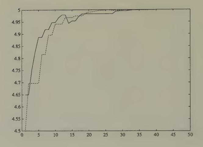
Figure 7:Simulation of saving rates for constant-gain algorithm when , . The gain is being held constant at 0.3 for each class of agents. Convergence is fast to the rational expectations savings rates.
Parametric and non-parametric adaptation
In the preceding formulation, people choose one saving rate for each level of government expenditure. This specification was designed potentially to let the system eventually ‘learn’ the rational expectations equilibrium, in which the ‘state’ is the vector of government expenditures. By letting agents learn a distinct saving rate to apply for each , we are in effect letting them use a non-parametric specification to learn about a policy function .
There are two potential difficulties with this specification. First, the transition matrix may imply that some states are visited very infrequently. Observations from such states will roll in only slowly, making learning occur slowly. Of course, in terms of the unconditional expected utility of the agents, failure to learn about the correct thing to do in such infrequently visited states may cost little. Second, when the number of states is large, the specification of one saving parameter for each state will become burdensome, again because the observations per state will roll in slowly.
An econometrician’s or statistician’s solution to this problem would be to assume a parametric form for the saving function , where is a vector of parameters, of small dimension relative to , and then to use all of the observations to estimate . A recursive algorithm for estimating the parameters would use the gradient
and the Jacobian . A recursive algorithm would be
This algorithm uses each observation to estimate a more or less smooth function to be used to determine savings.
Use of a parametric form for the saving function raises the issue of approximation. Evidently a learning scheme that uses a parametric specification has a chance eventually of converging to a rational expectations equilibrium only if a rational expectations equilibrium can be supported by a saving function within the class of functions determined by . For many models, the chosen econometrically convenient function will not be compatible with the functions determined by a rational expectations equilibrium. In these situations, a learning scheme based on a parametric specification will, if it converges, converge to an approximate rational expectations equilibrium.[11]
Learning the hard way
In the preceding model, learning occurs between non-overlapping generations of grandparents to grandchildren, with the grandchildren adjusting their grandparents’ saving choice after observing the consequences of their grandparents’ choice.[12] This model requires little of agents in the way of ‘theorizing,’ at the cost of rendering their learning dependent on the behaviors and experiences of their predecessors.
When we extend the horizon beyond two periods, it becomes increasingly inconvenient to model learning in this way because we have to wait longer for the consequences of life-time savings behavior to be known. If we attribute some ‘theorizing’ to our agents, we can avoid the need to learn only from one’s predecessors’ complete life-time experiences.
Learning via model formation
To motivate an alternative model of learning in this environment, consider the Euler equation for a young agent’s saving decision within a rational expectations equilibrium:
where the conditional expectation is over the equilibrium distribution of the rate of return on currency, , conditional on the current value of the deficit . As earlier, is the saving rate when . One way to formulate the problem of learning is to suppose that there is a representative young agent within each generation who knows the utility function and how to compute the derivative , but who does not know the distribution with respect to which the conditional expectation is to be computed in (31). To cope with this situation, the agent forms a model of the probability distribution with respect to which is to be computed, and adopts an algorithm for updating this distribution as new data arrive. At each point in time, the agent uses this estimated model distribution as the distribution in (31), and uses (31) to determine . Then the price level is determined as above, namely, by
We describe two methods for modelling and updating the required distributions.
Updating histograms
Here the agent’s model is created by simply forming histograms of ex post realized rates of return , one for each of the possible realized values of . When is observed at time , the young agent forms by using that histogram to represent the conditional expectation in (31). Let , , be the population of values of that have been observed prior to to follow the event , where is the number of times the event has occurred prior to time . Then is the value that solves
As time passes, the histograms are updated.
A parametric model of conditional probabilities
Here the agent adopts a parametric model of the conditional probabilities, namely,
At time the agent has an estimate of the parameters of the distributions , and uses them to determine behavior via the following approximation to (31):
As data on pairs flow in, the agent uses an adaptive algorithm to update his estimates of . For example, for each , let the distribution be a two-parameter distribution determined by the first and second moment. Then the agent would update these parameters using the stochastic approximation algorithm
where there is a different ‘clock’ for each event .
Approximate equilibria
When we adopt a learning scheme that restricts agents’ decision rules to too small a class of functions, we cannot expect the economy with adaptively learning agents ever to converge to a rational expectations equilibrium. The most we can hope is that the learning economy might converge to an approximate equilibrium, a concept that is used by applied researchers interested in computing rational expectations equilibria. In this section, I briefly describe some of the connections between algorithms to compute approximate equilibria and economies populated by adaptively learning agents.
Computing an equilibrium of the model becomes more demanding as we expand the dimension of the state space. Suppose that we modify the previous model by assuming that government expenditures are determined by the continuous state Markov process with transition kernel
All other aspects of the model remain unchanged. We conjecture an equilibrium saving function of the form , and use the equilibrium conditions to derive restrictions on this function. The household’s first-order conditions evaluated at can be written
where . The equilibrium condition and the government budget constraint imply , which can be solved for :
Substituting this into the household’s first-order condition gives
which is a functional equation in .
There exist a number of methods for solving a functional equation like (41) numerically. All of these methods replace the function with a finite-parameter approximation , then find values of the parameters that come as close as possible to satisfying (41).[13]
Method of parameterized expectations
Here is how Albert Marcet’s method of parameterized expectations can be used approximately to solve the functional equation (41). For convenience, write the right side of (41) as where .[14]
Guess that the conditional expectation on the right side of (41) has a form . Pick a starting value of , call it for . Use this guess and (41) to solve for an initial saving function .
Use a random number generator to draw a realization of length from the Markov process . Use this simulation and to generate a realization of . Then use this realization to compute the non-linear regression coefficients in the regression .
Solve the first-order condition for a new saving function .
Iterate on steps 1--3 to convergence.
There is evidently a close connection between this method for equilibrium computation and the behavior of a system populated by adaptive agents. Indeed, we can reinterpret a recursive or ‘on-line’ version of this algorithm as a system with adaptive agents. Thus, a recursive version of the nonlinear least squares algorithm is
where is the gradient of with respect to the parameters . Upon noting the resemblance between this algorithm and the learning scheme (41), it is understandable that Marcet proposed his equilibrium computation scheme as an outgrowth of earlier work on the dynamics of least squares learning systems.
Learning and equilibrium computation
Learning algorithms and equilibrium computation algorithms look like each other. Equilibrium computation algorithms often have interpretations as centralized learning algorithms whereby the model builder, acting in a role of ‘social planner,’ gropes for a set of pricing functions for markets and decision rules for agents that will satisfy all of the individual optimum conditions and market-clearing conditions. We have also seen that learning systems with boundedly rational agents sometimes have interpretations as decentralized equilibrium computation algorithms.
Recursive kernel density estimation
A continuous state (for ) specification in the present model is a convenient context for describing another way to formulate learning nonparametrically, namely, via recursive kernel estimators of a kind studied by Chen and White (1993). To describe their formulation, we first recall the nature of kernel estimators. Suppose that we have observations , , on the -dimensional random vector drawn from an unknown joint density . Let be a probability density for , say a multivariate normal density. Then the kernel estimator of the density of is
where is a fixed ‘bandwidth’ parameter.
Chen and White study a modified recursive version of such estimators. They let be a sequence of bandwidths with , and be an arbitrary initial density. Then they construct the sequence of distributions via the stochastic approximation algorithm
For the present example, we could let . At time , we would let behavior be determined by the solution of a version of (31) in which the conditional expectation on the right side is evaluated with respect to the conditional distribution for conditional on that can be deduced from the joint density .[15]
Learning in a model of the exchange rate
We now study an environment for which the rational expectations equilibrium exchange rate is indeterminate, but we expel all rational agents and replace them with adaptive agents.[16] We endow these adaptive agents with learning algorithms and initial values for their decisions, which serve to render the exchange rate and all other endogenous variables determinate. We want to study how the exchange rate behaves, and whether a ghost of indeterminacy still lurks.
The economy consists of a sequence of overlapping generations of two-period lived agents. There are two kinds of currency, available in supplies and that are fixed over time. At each date , there are born a constant number of young agents who are endowed with units of a nonstorable consumption good when young, and units when old. A young agent makes two decisions. First, he chooses an amount to save when young. Second, he chooses a fraction to allocate to currency 1, and allocates the remainder to currency 2. At time the young agent’s realized utility from those decisions will be
where is the price level at time in terms of currency , and is the gross rate of return on currency . Here is an increasing and strictly concave function of consumption of the one good. In the examples below, we shall set . We calculate the gradient
We also use the elements of the matrix of second partials.[17] For the purposes of studying learning, the economy consists of two subsequences of agents. Each subsequence is identified with a class of agents, whom we dub ‘odd’ and ‘even.’ As in the preceding model, we have two clocks , one for odd and the other for even agents, that count only two-period episodes used to evaluate realized utility. Let be a sequence of positive numbers satisfying . The values of for each class of agents evolve according to the recursive algorithm
There are two realizations of this algorithm, one for the odd agents, the other for the even agents. Agents of each class thus learn from the utility experience only of previous agents of their own class.[18] The price level is determined by
In odd periods, the pair for the odd agents is used in (51), while in even periods, the pair for even agents is used in (51) to determine price levels in terms of the two currencies.
Given initial conditions for for each class of agents, equations (46), (49), (51) determine the evolution of the decisions , and the prices in terms of the two currencies. The exchange rate is just .
Figure 8 and Figure 9 report the results of simulating this system starting from two different sets of initial conditions for , but common initial conditions for the ’s.[19] For each experiment, the exchange rate path rapidly converges to a constant value, but the limiting exchange rate values differ between the two economies. Evidently, the exchange rate depends sensitively on the initial conditions that we choose. Figure 10 shows saving rates for the two types of agents in experiment 1, while Figure 12 displays the evolution of their portfolio parameters . All of these parameters are gradually converging to values consistent with a rational expectations equilibrium.
Figure 8:Logarithm of exchange rate in experiment 1.
Figure 9:Logarithm of exchange rate for experiment 2. Experiments 1 and 2 share identical parameters, except for the initial conditions on for odd and even agents.
Figure 10:Saving rate for odd agents in experiment 1.
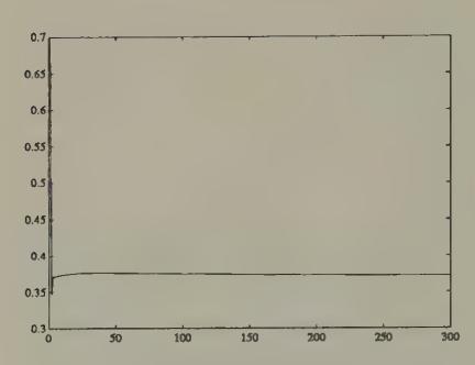
Figure 11:Saving rate for even agents in experiment 1.
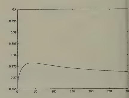
Figure 12: for odd agents in experiment 1.
Exchange rate initial-condition dependence
For the purpose of understanding the sense in which this system can render the exchange rate determinate, it is useful to consider the limiting properties of algorithm (49). If algorithm (49) comes to rest, it will, as it is designed to do, come to rest at a point at which . The condition implies , or , where is the gross rate of return on currency . This is the same arbitrage condition that leads to exchange rate indeterminacy under rational expectations. The reasoning that underlies the exchange rate indeterminacy under rational expectations also implies that the rest points of algorithm (49) leave the exchange rate unrestricted. Our learning system renders the exchange rate path determinate by having the ‘dead hand of history’ put enough sluggishness into decisions. The exchange rate path can be said to be ‘history-dependent’ because the initial conditions assigned to assume an importance that does not vanish as time passes.[20] [21]
The no-trade theorem
Jean Tirole (1982) proved a sharp ‘no-trade’ theorem that characterizes rational expectations equilibria in a class of models of purely speculative trading.[22] [23] The equilibrium market price fully reveals everybody’s private information at zero trades for all traders. The no-trade theorem overrules the common-sense intuition that differences in information are a source of trading volume.
The remarkable no-trade outcome works the rational expectations hypothesis very hard. This is revealed clearly in Tirole’s proof, which exploits elementary properties of the (commonly believed) probability distribution function determined by a rational expectations equilibrium. In this section, I describe how backing off rationality can (temporarily) undo the no-trade result, and produce a model of trading volume. I first describe an environment for which the no-trade theorem holds under rational expectations, then withdraw Tirole’s rational agents and replace them with Robbins--Monro adaptive agents.
The environment
The environment is one analyzed in detail by John Hussman (1992).[24] There is a competitive market for a stock that is a claim on a dividend process governed by
where , , and is a vector white noise. There are two classes of traders, dubbed and , present in equal numbers (for convenience we’ll assume one each) who have different information about dividends. At time , traders of both classes observe the history of the publicly available information . In addition, traders of classes and , respectively, observe the pieces of ‘private information’:
where are white noises that are orthogonal to each other and to each component of . At time , traders of class observe a history generated by the information vector .
Traders behave myopically, each period maximizing the one-period utility function
subject to
where is a constant gross interest rate on a risk-free asset, is agent ’s information set, and is agent ’s purchases. This leads to a demand function for trader of class that is linear in the expected ‘excess return’:
where ; is the variance of conditional on the information set ; and is the excess return of the stock over the risk-free asset.
Following Tirole, we assume that the asset is available in fixed supply , which for convenience we assume to be zero.[25] A rational expectations equilibrium is a stochastic process for that satisfies the market-clearing condition
Prices fully revealing with no trade
For ease of exposition, we shall assume that in forming conditional expectations, agents of both classes condition only on the most recent observation , which means that we set . Hussman (1992) and Sargent (1991) describe how to set things up to condition on the (infinite) history of . We also replace conditional expectations with linear regressions, a step we can defend by one of two standard justifications.[26] Substituting the demand functions (59) into equilibrium condition (60) gives
or
where the random variable measures the excess return of the stock over the risk-free asset. Writing the regressions , (62) implies
Because we have assumed that the information vector , (63) can hold only if both sides are constant over time. However, (62) with , a constant implies .[27] Substituting into the demand functions shows the no-trade outcome. The condition that shows that the market price adjusts to reveal fully all of the private information that is relevant for predicting excess returns.
Models with ‘noise traders’ break the no-trade theorem by replacing (60) with , where is an exogenous stochastic process of supplies by the noise traders. Technically, notice how the presence of a time-varying, random process disrupts the argument leading to (62).
Computation of the equilibrium
In order both to study the rational expectations equilibrium in more detail and to provide a framework from which we can expel rational agents and resettle adaptive agents, it is useful to have a way of computing the rational expectations equilibrium. We follow Hussman and adapt the apparatus of Marcet and Sargent (1989b) to this purpose. A trader of type observes the history of , fits the vector autoregression,[28]
and uses it to forecast the components of :
Then trader ’s estimate of excess returns is
where .
The state vector and the innovation vector for the market are
Using (66) and the equilibrium condition (60), we can derive a state transition equation of the form
where , are matrix functions of that are described by Hussman. The form of (68) emphasizes how traders’ perceptions of the laws of motion, as parameterized by the vector autoregressive parameters , influence the law of motion for the entire state .
Since is a subvector of , system (68) can be used to deduce the projections
where depends on and the moments . Thus, we have a mapping from a pair of perceived laws of motion to a pair of matrices that determine optimal (linear least squares) predictors. A rational expectations equilibrium is a fixed point of this mapping.
Tampering with the no-trade theorem
The no-trade theorem follows directly from the equality
and in particular from the facts that , are each constant over time, and that , are each a conditional expectation of the same random variable, conditioned on different information sets, but calculated with respect to the same joint probability distribution. We can temporarily disrupt the forces leading to the no-trade theorem by withdrawing from our agents knowledge of the (equilibrium) joint probability distributions required to compute , and giving them instead initial conditions for in their vector autoregressions and a recursive algorithm for updating their estimates of .[29] The effect of this will be to replace (63) with an equilibrium condition of the form
where . The facts that in (71) are time-dependent, and that they start from arbitrary initial conditions, raises the possibility that , so that trade will occur.
The system’s motion is described by
where , and the first equation is formed simply by replacing by in (68). To start the system, we need initial conditions for for . We shall start the system from initial conditions in the vicinity of a rational expectations equilibrium.
Some experiments
Figure 13, Figure 15, and Figure 17 report some simulations of the system with least squares learning.[30] Figure 13 plots the price and volume from a simulation of a system with least squares learning, where the system has been initiated with beliefs that are perturbed by very small amounts from the rational expectations beliefs, and the covariance matrices (the ’s) have been set close to those from the asymptotic distribution theory that governs the regression of someone who had lived for 100 periods in the rational expectations equilibrium. These graphs illustrate how the price with least squares learning resembles the rational expectations price, but diverges enough from it to generate volume. Hussman and Sargent studied the behavior of such systems over much longer horizons, and found that over time the gap between the rational expectations price and the price under least squares learning vanishes, and so does volume. But positive trading volume persists for a very long time.
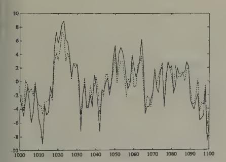
Figure 13:Rational expectations price (solid line) and price under least squares learning (dotted line) after 1000 periods of learning, with initial beliefs close to those appropriate for a rational expectations equilibrium.
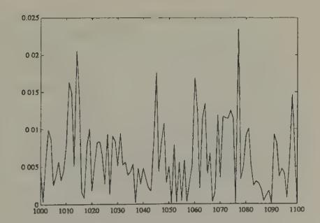
Figure 14:Volume with least squares learning after 1000 periods.
Figure 15 and Figure 16 plot parts of a simulation of the same model with initial beliefs that assign too much weight to the market price in determining expected excess return. In particular, initial beliefs are equal to the rational expectations beliefs except that the coefficients on current price in the vector autoregression determining expected excess return are raised in absolute value by 40 percent vis à vis their rational expectations values. The initial 150 periods of the simulation are plotted in Figure 15, while Figure 17 plots observations after 1000 periods. These figures indicate how we can make prices temporarily diverge from their rational expectations values by driving initial beliefs farther away from the rational expectations values. Figure 17 shows how, with the passage of time, least squares beliefs are adapting to eliminate differences from rational expectations.[31]
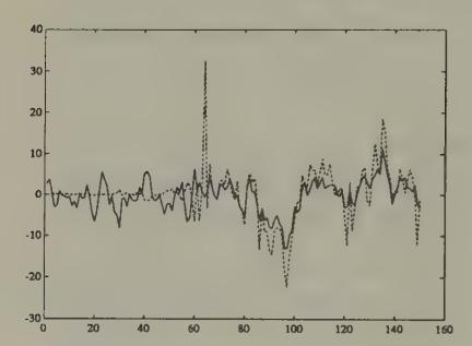
Figure 15:Rational expectations price (solid line) and price under least squares learning (dotted line), starting from beliefs that overweight the market price: first 150 observations.
Figure 16:Volume under least squares learning, starting from beliefs that overweight the market price.
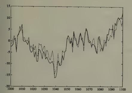
Figure 17:Rational expectations price (solid line) and price under least squares learning (dotted line), starting from beliefs that overweight the market price, after 1000 periods of learning.
Figure 18:Volume under least squares learning, starting from beliefs that overweight the market price, after 1000 periods of learning.
Sustaining volume with a constant gain
We can prevent convergence to rational expectations and extinction of volume by assigning agents constant-gain (i.e., ) versions of the recursive algorithm. By setting , we can control the neighborhood of a rational expectations equilibrium, and the average level of volume to which this model would eventually converge.
Using a constant-gain algorithm might be a good idea for agents who take time invariance of their forecasting model with a grain of salt, and who place a premium on adaptability. Second, constant-gain algorithms assign enough greater weight to recent observations than ordinary least squares to defeat the forces that generate consistency of ordinary least squares under classical conditions. The stay-on-your-toes spirit of constant-gain algorithms can have advantages in situations (like this no-trade model with least squares learning) in which one is fitting a time-invariant model where the law of motion is really time-varying.[32]
In giving up the ability to converge, the constant-gain adapter retains an ability to keep up with the times.[33]
Learning with an infinite horizon
We have already encountered a couple of situations in which agents want to set their behavior to satisfy an Euler equation, and where they only need to learn about the distribution with respect to which to compute the expectations that appear in their Euler equation. I described how we could have applied this setup to the Markov deficit example, and we actually did the no-trade example in this way. In those examples, because of the short horizons of the agents, there were alternative ways to model learning, e.g. by letting agents ‘learn the hard way’ by observing the past utility-experiences associated with the dynamic plans of their predecessors. Where agents have infinite planning horizons, we are more restricted in how we can model agents’ learning.
To illustrate learning (with coaxing) in a simple infinite-horizon context, this section describes least squares learning in the context of a linear version of Lucas and Prescott’s equilibrium model of investment under uncertainty, an example studied by Marcet and Sargent (1989a). This example has the following features:
(a) Because the horizon is infinite, agents in the model get a lot of coaxing. The model is set up so that agents know most of what they require to make optimal decisions, and only learn about a limited aspect of the system, namely, the law of motion involving an aggregate endogenous state variable. Firms know enough to form and solve their Euler equation, but don’t know the equilibrium conditional distribution of the future values of the output prices that appear on the right side. Firms use a recursively updated estimate of a vector autoregression to solve their Euler equation.
(b) Verifying the convergence of the system is technically difficult because the firms are learning about a ‘moving target,’ a law of motion that is influenced by their own learning behavior.
Investment under uncertainty
A representative firm chooses its capital stock to maximize
where , , , and where is the price of a single commodity. The price of the commodity is determined in a competitive market. The demand for the commodity is governed by
where is the average level of capital used to produce output in this market (so that average output is ), and is a serially uncorrelated random process with mean zero. Under rational expectations, the firm is supposed to know the law of motion for average capital, namely,
and to use it in conjunction with (76) to forecast prices. Under the assumption that the firm knows the laws (76), (77) governing prices and the market-wide average capital stock, the firm’s problem can be represented as a dynamic programming or discrete-time calculus of variations problem. The Euler equation associated with this problem is
where is the conditional expectation evaluated with respect to the equilibrium distribution generated by (76), (77).
Rational expectations equilibrium as a fixed point
For given values of , in (76), the prediction problem associated with the right side of the Euler equation (78) can be formulated as follows. Represent (77) as
or
where . Using (80) to evaluate the conditional expectation, the Euler equation can be represented as
Equation (81) summarizes individual firm behavior under the beliefs (77) about the aggregate state . We impose equilibrium by setting , and solving the resulting equation for the actual law of motion for induced by the beliefs (77). We obtain
where
This construction induces a mapping from a perceived law of motion for into an actual one. When firms believe that the law of motion is (77), they act to make the actual law of motion (82). A rational expectations equilibrium is a fixed point of this mapping, namely, a pair that satisfy
Least squares learning
Marcet and Sargent (1989a) describe a version of this model with adaptive agents. Firms formulate and recursively estimate an autoregression of the form (77), using the stochastic approximation algorithm
Firms’ behavior is determined each period by using the estimated vector autoregression to evaluate the conditional expectation on the right side of the Euler equation (77). This behavior causes the actual evolution of the capital stock to be
Technically, this example has many of the features of Bray’s model, with the additional feature that, even in the rational expectations equilibrium (i.e. the system without learning), there is a state variable, , that imparts dynamics to the system.
It is about the law of motion of that state variable, and not a fixed mean, that the firms are learning. Nevertheless, very similar considerations govern the convergence of this system to a rational expectations equilibrium.
Marcet and Sargent (1989a) applied methods developed by Lennart Ljung (1977) to describe the sense in which the limiting behavior of the stochastic difference equations (85), (87) is governed by the associated ordinary differential equations
where , from system (82), evaluated at the fixed vector . Notice that the rest points of this system are rational expectations equilibria. Stability of this ordinary differential equation system about the rational expectations equilibrium is a necessary condition for the (almost sure) convergence of the stochastic difference equations (85), (87) to the rational expectations equilibrium. Sufficiency is more tenuous and troublesome.[34] [35] Marcet and Sargent studied the technical complications that the presence of learning about a law of motion for an endogenous state variable like added to the sort of system studied by Bray.
Convergence theorems
I now briefly describe a method that has been used to analyze the limiting properties of models in which the agents’ behavior is determined by their use of adaptive estimators. Such systems have the property that laws of evolution of the endogenous variables are determined in part by the adaptive estimation process. Because the agents are learning about a system that is being influenced by the learning processes of people like themselves, these systems are sometimes called ‘self-referential.’ That the adaptive estimators are not estimating the parameters of a fixed data-generating mechanism means that standard econometric proofs of convergence of estimators (e.g., their consistency and asymptotic efficiency) cannot usually be applied. Instead, another approach based on stochastic approximation methods has increasingly been used.
I shall illustrate the kind of analysis that can be done with stochastic approximation methods in the context of a particular example, namely our model with a stochastic government deficit.[36] Consider a version of that model in which agents are learning via a parametric model which they fit to the distribution of the return on currency. In particular, assume that agents generate forecasts of the rate of return on currency by fitting the parametric model
where is the time estimate of the vector of parameters in the probability model, and is a possibly nonlinear function mapping the government deficit into a forecast of the rate of return on currency between and , which we denote . We assume that agents use the following stochastic approximation algorithm for estimating :
where is the gradient of with respect to evaluated at and . Recall that (91) simply implements a recursive nonlinear least squares algorithm.
The model has the self-referential property that, when agents forecast according to the rule and when the ’s are updated according to (91), the optimal forecast has a form
where
where is the conditional expectation operator, is a function mapping into the least squares forecast , and is a random process with the property that is orthogonal to every (Borel measurable) function of .[37] The function , which depends on , is determined implicitly by the process of solving the model.[38]
Substituting (94) into (91), the recursive learning algorithm can be written
An associated ordinary differential equation
We want to study the behavior of the system formed by the assumed exogenous Markov process for government expenditures which together with equations (94) and (95) determines the evolution of . In particular, we want to find some conditions under which this system converges to an asymptotically stationary system in which the parameters determining beliefs stop moving. When convergence does occur, we want to describe the resulting limit point in terms of how it relates to the concept of a rational expectations equilibrium.
Application of arguments in the spirit of Ljung and Söderström (1983) and Kushner and Clark (1978) can be used to show that the limiting behavior of the system of stochastic difference equations defined by the Markov process for and equations (94) and (95) is determined by an associated system of ordinary differential equations. This associated differential equation is derived by conducting the following mental experiment. Temporarily suspend the operation of system (95), and consider the system operating with a fixed for ever. Assume that this system converges to a unique invariant distribution,[39] and let be the conditional expectation of evaluated with respect to this invariant distribution. Form the associated differential equation system:
where is the unconditional expectation operator evaluated with respect to the asymptotic stationary distribution associated with the fixed parameter vector . The system of ordinary differential equations (97) is formed mechanically by taking expectations of the objects ‘to the right of ’ in equation system (95), and using the resulting expectations to estimate the average motion of over small intervals of time . The expectations are taken with respect to the stationary distribution associated with a fixed .[40]
We also consider the smaller ordinary differential equation system
Propositions
Several properties of systems like this have recurred in a variety of contexts, among the important ones being:
(a) The rest points of the ordinary differential equation (o.d.e) system (97) satisfy
If the support of includes a rational expectations equilibrium, the first equation of (100) can be satisfied by , in which case we have a rational expectations equilibrium as a rest point of (97) or (99). If the support of does not include a rational expectations equilibrium, then the first equation of (100) identifies a set of orthogonality conditions that are the first-order necessary conditions for a special approximation problem. If the function were independent of (which it usually is not), then these equations would be orthogonality conditions for the problem: find the value of which makes the function best approximate the fixed function , where the approximation criterion is the mean square difference between the functions
The approximation problem is unusual because determines the approximating function and also influences the function being approximated . This aspect of the approximation problem reflects the self-referential property of the system.
(b) If the estimators converge, they converge to a rest point of the ordinary differential equation (97).
(c) If a fixed point of the ordinary differential equation (97) is locally unstable, then the estimator cannot converge to that fixed point.
(d) Suppose that the ordinary differential equation (97) is globally stable about a unique rest point. Then there exists a modification of the recursive algorithm for , which converges almost surely to the rest point.[41]
(e) Convergence theorems require that look like . Convergence will not occur with ‘constant-gain’ versions of the algorithm.[42]
(f) Few results are available on rates of convergence. However, theorems described by Benveniste, Métivier, and Priouret (1990) can sometimes be used to show that a necessary and sufficient condition for -convergence of to the fixed point is that the eigenvalues of the Jacobian of the linear approximation to the small o.d.e. (99) at the fixed point are all less than in modulus. Notice that this condition is stronger than the necessary condition for ‘local stability’ of the algorithm at the fixed point, namely that the eigenvalues of this same linear approximation are less than 0 in modulus.
Propositions like (a), (b), (c), and (e) are not difficult to obtain, and can be expected to apply across a wide variety of models, both linear models like those studied by Marcet and Sargent (1989a, 1989b, 1992) and nonlinear ones like the ones studied by Woodford (1990). Propositions like (d) are harder to obtain, and often involve delicate and involved computations to verify assumptions sufficient to assure almost sure convergence. The amount of work to be done depends on the details of the device that is used to force the algorithm infinitely often into the domain of attraction of a fixed point. So far very little formal work has been done along the lines of proposition (f) about rates of convergence.[43] [44]
Conclusions
The examples in this chapter all take an environment that had been studied under rational expectations and add a source of transient dynamics coming from adaptive least squares learning. The dynamics are transient because the ‘fundamentals’ in these environments are time-invariant, and because the adaptive algorithms we have given our boundedly rational agents eventually settle upon good time-invariant decision rules for those environments.[45]
Are transient dynamics created in this way likely to be a useful addition to the list of ways that applied economists have of inducing dynamics? Among the principal mechanisms through which applied economists induce dynamics are:
(a) Capital (physical and human).
(b) Costs of adjustment.
(c) Serially correlated exogenous processes and disturbances.
(d) Information structures that induce agents to solve signal extraction problems or incentive problems.
I suspect that it is too early to add the sort of transient dynamics described in this chapter to this list of workhorses in applied economic dynamics. However, the examples in this chapter can teach us various things.
Beyond exhibiting the structure of a model of market equilibrium with dynamic supply behavior under least squares learning, Bray’s model displays circumstances under which at least one class of plausible adaptive algorithms eventually converges to rational expectations.
The model with a stochastic government deficit sensitizes us to the issue that how fast adaptive agents can be expected to learn to have rational expectations depends on how complicated is the stochastic environment they must learn about, and how much prior information they are endowed with by way of a parametric form to learn about. In particular, how fast adaptive agents learn depends on how complicated is the government policy regime.
Adaptive algorithms are in principle capable of resolving indeterminacies in some rational expectations models like our exchange rate model, but in a very tenuous way. In our exchange rate example, the equations determining the limiting behavior of the system leave the exchange rate indeterminate (because those equations just recover the logic of exchange rate indeterminacy), but the adaptive algorithms assign enough force to initial conditions and to ‘history’ to determine the exchange rate path. By sufficiently tying down the expectations process that was left underdetermined by the rational expectations equilibrium, the adaptive mechanism selects an exchange rate path. This may seem a weak reed on which to base exchange rate determination.[46]
Adaptive learning provides enough friction temporarily to break the logic of the no-trade theorem, and so to provide a model of trading volume. This is one of a class of examples in which incorporating adaptive agents would serve, at least temporarily, to modify or take the edge off very sharp predictions that arise in some rational expectations models. One can imagine using similar shading of sharp rational expectations results in particular environments giving rise to Ricardian or Modigliani--Miller results for government monetary-fiscal operations.
A comparison of the Marcet-Sargent example with some of the earlier ones shows that there are many choices to be made in endowing our artificial agents with adaptive algorithms. These choices supply differing amounts of ‘coaxing’ to our boundedly rational agents.
In the next two chapters I shall describe more potential uses of models of bounded rationality.
This model has the special feature that, in the rational expectations equilibrium, the unconditional expectation equals the conditional expectation, a consequence of there being no time-varying state variables in the rational expectations equilibrium.
Marcet and Sargent (1989a) show that the limiting behavior of is governed by the associated differential equation , which is stable for . The right hand side of this differential equation can be expressed as , where is the mapping from the perceived forecast of prices to the optimal forecast of prices . Stephen DeCanio (1979) and George Evans (1985, 1989) used the operator to define a notion of expectational stability. Marcet and Sargent (1989a) described a sense in which the operator governs the convergence of least squares learning schemes in a class of models.
Jasmina Arifovic (1991) has studied a version of Bray’s model in which Bray’s representative least squares learner is replaced by a population of heterogeneous agents with heterogeneous beliefs. She applied a genetic algorithm to this environment, and found that the population can sometimes learn its way to a rational expectations equilibrium even when Bray’s necessary condition is violated.
See Mark Feldman (1987) for a study of the convergence of a model with a collection of Bayesian agents who start out with divergent priors. Also, see El-Gamal and Sundaram (1993).
Marcet and Sargent (1989b) describe systems with heterogeneous beliefs in which heterogeneity remains in the rational expectations equilibrium because people are assumed to be differentially informed.
Models of this class typically have equilibria outside the class of stationary ‘fundamental’ equilibria that we are focusing on. In addition to a class of non-stationary equilibria that David Gale (1973) studied, Azariadis, Guesnerie, Cass and Shell have studied sunspot equilibria for such models. Michael Woodford (1990) and George Evans (1989) have studied how collections of agents using least squares learning schemes can converge to a sunspot equilibrium. To study this question, Evans used a distinction between ‘strong’ and ‘weak’ expectational stability, which focuses on whether or not convergence is robust to failure to specify the order of the perceived autoregressive moving average process in a way that is overparameterized with respect to an equilibrium process. ‘Strong stability’ is the property that convergence to a rational expectations equilibrium occurs when agents overparameterize the law of motion they are learning about.
See Cass and Shell (1983), Azariadis (1981), and Azariadis and Guesnerie (1986).
In models with agents who have an infinite horizon, it will obviously not work to let agents see and base adaptation of decisions on realizations of the infinite-horizon utility functional. Adaptation in settings with infinite-horizon agents has been modelled by endowing agents with versions of ‘adaptive control’ algorithms in which adaptation is confined to learning about a rule for forecasting state variables that are not controllable by the agent. The agent simply resolves a dynamic programming problem at each point in time with a revised forecasting rule. See Marcet and Sargent (1989a, 1989b) for some examples of such setups.
The initial conditions for the saving rates can be read from the graphs.
See Evans and Honkapohja (1993b) for a discussion of some of the features of constant gain algorithms.
See Marcet and Marshall (1992) and Sargent (1991). Also, see Kenneth Judd (1990, 1992) for descriptions of a variety of numerical methods for computing approximate equilibria.
A byproduct of setting things up in this way is the alternation of turns between odd and even sets of agents. This ‘two-population’ feature of the learning algorithm duplicates or resembles the experimental environments of Marimon and Sunder (1992) and Arifovic (1993), to be discussed in the next chapter.
See Kenneth Judd (1992) for a critical survey of and guide to such methods.
See Marcet and Marshall (1992) for a formal analysis of the algorithm.
Chen and White (1992, 1993) have attained results on rates of convergence of such nonparametric estimators under assumptions permitting less feedback from agents’ behavior to outcomes than the present example admits.
The environment is the one studied by Kareken and Wallace (1981).
These are given by ; ; .
Algorithm (49) can be modified to incorporate ‘simulated annealing’ by replacing by everywhere in the algorithm, where is a random variable with mean zero. We can implement a so-called ‘constant-gain’ algorithm by setting , a constant. A constant-gain algorithm with and with the initial value of set equal to the Hessian implements Newton--Raphson.
We set the parameters of the model at , , , .
It is possible to construct stochastic versions of this model in which the exchange rate is path-dependent in the sense that realizations emanating from identical initial conditions would eventually converge to different exchange rates because of the different realizations of the random processes impinging on the system’s transient dynamics.
Evans and Honkapohja (1993) describe how adaptive learning rules resolve equilibrium indeterminacy problems: ‘models with multiple solutions are converted into models with path dependence in which the trajectory of the economy, and the [rational expectations equilibrium] attained in the limit, are determined through a learning rule by initial forecasts and by the sequence of exogenous shocks.’
‘Purely speculative trading’ means that all insurance and consumption-smoothing reasons for trading are assumed absent.
Milgrom and Stokey describe a related no-trade theorem.
Hussman’s work is related to work by Jiang Wang (1990). For other work on methods of circumventing the no trade theorem, see Harald Uhlig (1992).
The important thing is that the supply is fixed over time.
Either assume that all distributions are multivariate normal or restrict decision rules to be linear.
The vector is the innovation vector.
The work described in this section is from Hussman and Sargent (1993).
Parameter values were set at , , , . Constants have been omitted from the dividend process, with the consequence that equilibrium prices fluctuate around zero. By adding constants, we could make prices fluctuate around a positive number.
The price differences show higher-than-normal kurtosis, which decreases toward three as the system converges to a rational expectations equilibrium.
In the model of Sims and Chung to be described in Chapter 7, we shall see a situation in which using a ‘random coefficients’ specification enhances a government policy-maker’s adaptability and sometimes leads to superior outcomes, relative to those implied by ‘decreasing-gain’ specifications.
There are alternative ways to break the no-trade theorem. One class of alternatives would alter the environment to restore non-speculative motives for asset trades, e.g. via endowment heterogeneity coupled with consumption smoothing motives. Another class of explanations would retain the only-speculative motive assumption, but would model trading processes explicitly in such a way that positive volume and lack of full revelation of information would be the outcome of implementing one of the auction mechanisms analyzed, say, by Gresik and Satterthwaite (1989). I don’t know whether the learning route described in the text is more promising than these alternatives.
The sufficient conditions for convergence that have been discovered to date involve adding some side conditions to the least squares algorithm designed to insure that the altered algorithm visits the basin of attraction of the fixed point of the operator infinitely often. See Ljung (1977), Ljung and Söderström (1983), and Marcet and Sargent (1989a) for a discussion of various ways of modifying the algorithm. What is needed to get the stochastic approximation approach to yield almost sure convergence to a fixed point of the o.d.e. is some device that assures that the algorithm infinitely often visits the domain of attraction of the fixed point of the o.d.e.
Marcet and Sargent also study the sense in which the local stability of the learning scheme is governed by the smaller o.d.e. .
This section is based on Marcet and Sargent (1989a) and Woodford (1990). Bullard and Duffy (1993) study least squares learning in an economy with overlapping generations of -period lived agents. For , they find that least squares learning fails to converge locally to a rational expectations equilibrium. Also see Bullard (1991) for a discussion of how complicated nonlinear dynamics can sometimes emerge out of least squares learning.
This property of identifies as the conditional expectation function.
i.e., a unique asymptotic stationary distribution.
Notice the ‘mean field theory’ flavor of this approach: approximating deterministic dynamics are being used to study aspects of an underlying stochastic process.
The modifications are devices that ‘project’ the estimator back into the intersection of the domain of attraction of the fixed point with the set of values of for which the system converges to an asymptotically stationary distribution for , . See Ljung (1977), Ljung and Söderström (1983), and Marcet and Sargent (1989a) for a discussion of various ways of modifying the algorithm. What is needed to get the stochastic approximation approach to yield almost sure convergence to a fixed point of the o.d.e. is some device that assures that the algorithm infinitely often visits the domain of attraction of the fixed point of the o.d.e.
The most that can be hoped for with constant-gain versions of the algorithm is convergence in a stochastic sense of visiting a specified neighborhood of a fixed point of the o.d.e. with a relative frequency that depends, among other things, on the gain parameter .
See Marcet and Sargent (1992) for an analysis of rates of convergence in a particular model, with part of the analysis being based on the theorems of Benveniste et al., and another part being based on Monte Carlo methods. Also see Ljung, Pflug, and Walk (1992).
See Chung-Ming Kuan (1989) and Mohr (1990) for useful early contributions. Marcet and Sargent (1993) state a proposition about a rate of convergence.
The exceptions are the constant-gain algorithms.
Put differently, a regime that allows the exchange rate to be history-dependent seems to be an ill-formed mechanism.