6. Experiments
Interpreting experiments
Arthur (1991) and Rust, Palmer, and Miller (1992) have used adaptive algorithms to mimic and interpret the behavior of human subjects in experiments. In this chapter we describe some experiments that have been performed on two models of monetary economies that appeared in earlier chapters. Among the goals of the experimenters was to shed light on the quality of guidance supplied by rational expectations and adaptive dynamics in selecting among multiple stationary equilibria. The first example is an overlapping-generations monetary economy with two stationary equilibria. The second is the exchange rate model with indeterminate equilibria.
A model of inflation
Marimon and Sunder (1992) put human subjects in an experiment designed to mimic a model with multiple equilibria that had been studied by Sargent and Wallace, Bruno and Fischer, and Marcet and Sargent.[1]
In this model, the ‘rational expectations dynamics’ and the ‘adaptive dynamics’ share common rest points but assign opposite stability characteristics to those rest points. Marimon and Sunder’s goal was to study how the experimental observations would match these different theoretical dynamics.
The environment
The model is a nonstochastic version of the overlapping-generations model with government expenditures described in the previous chapter. At each date there are ‘born’ a constant number of young people, each of whom is endowed with of a consumption good when young, and units when old. Subjects have ex post utility measured by
and they can exchange consumption when young for consumption when old according to the budget constraints,
where is the price level at time , and is currency held from to .
A government issues an unbacked currency and uses it to finance a constant per-young-person deficit . The government’s budget constraint is
where here is the supply of currency per young person. Each period, the price level is determined in a market in which the young trade some of their consumption goods to the old for currency.
Rational expectations solution
The fundamentals of this economy are not random. With perfect foresight about the price level, the saving function of the young is
where is the gross rate of inflation. The government’s budget constraint can be represented as
where . The equilibrium condition is . Equating to in (5) and (6) and eliminating gives the autonomous difference equation in :
where , , . The function , which is graphed in Figure 1, determines the rational expectations dynamics of .
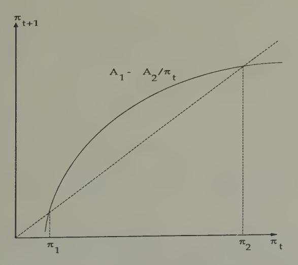
Figure 1:The equilibrium law of motion of the inflation rate. The curved line shows the equilibrium inflation rate in period , , as a function of the inflation rate in period . The dotted line is the 45 degree line. The intersections of the curved line with the 45 degree line are stationary equilibrium inflation rates. An increase in lowers the curve .
Figure 1 indicates that, if there exists an equilibrium, then there exist two stationary equilibria and a continuum of nonstationary equilibria. Evidently, of the two stationary equilibria, the one with the lower inflation rate is unstable under the rational expectations dynamics, while the one with the higher inflation rate is stable. The curve shifts downward with an increase in , because is decreasing in . The comparative statics of the (unstable) lower stationary inflation rate are ‘classical’ in the sense that increases in increase the stationary inflation rate. The comparative dynamics of the higher stationary inflation rate are anti-classical, a permanent increase in causing the stationary inflation rate to fall because the economy is on the wrong side of a ‘Laffer curve’ in the inflation tax rate. Despite the fact that many classical doctrines in monetary theory depend on selecting the lower stationary equilibrium inflation rate, the rational expectations dynamics selects the higher one. The stationary equilibrium associated with the lower inflation rate Pareto-dominates all of the other equilibria, stationary or nonstationary. Thus, the rational expectations dynamics repels from the Pareto-optimal solution.[2]
The least squares dynamics
Marcet and Sargent (1989c) studied a version of this model in which people form forecasts of next period’s price level using a least squares regression of price on the once lagged price.[3] The system with least squares learning has the same two stationary inflation rates as the system under rational expectations. However, Marcet and Sargent showed how the least squares dynamics reverses the stability of the two stationary equilibria: under the least squares dynamics, the lower stationary inflation rate is the limit of the dynamics for almost all starting values, if any limiting value exists.[4] Bruno and Fischer (1990) discovered similar outcomes in a closely related model in which they replaced perfect foresight with a version of Friedman’s adaptive expectations mechanism.
Marimon and Sunder’s experiment
Marimon and Sunder (1992) designed an experimental environment to implement this economy. They put a fixed number of participants in sessions of length periods, unknown to the participants, but chosen according to rules, known to the subjects, that made the economy equivalent from participants’ point of view to one that never ends. At each period , of the subjects were designated as ‘young,’ meaning that they were given an opportunity to submit a saving schedule telling the time price level (or its reciprocal, the value of money in terms of goods) at which they were willing to supply time output to the old for money in discrete amounts [5] Marimon and Sunder linearly interpolated between integers to get an individual’s supply schedule, then summed across the young to get total supply. To determine the time price level, they set this supply schedule against a total demand schedule, composed of the sum of the demands for goods from the government and the old.[6]
Subjects were randomly selected to be born or born again as young. Each period there were young, old, and agents temporarily sitting on the sidelines, awaiting rebirth. A participant was rewarded proportionately to his accumulated value of the criterion (1). In addition, those who sat on the sidelines participated in a ‘forecasting game’ from which they received additional rewards. At the beginning of each period, those on the sidelines were asked to forecast the market-clearing price for that period. The author of the forecast that came closest to the actual time price was awarded a prize, and the winning forecast was announced to all subjects at the end of the period, together with the equilibrium time price.
A session ended after forecasts for period had been turned in, at which point Marimon and Sunder announced that the economy had ended at . Marimon and Sunder then redeemed money holdings of the time young at a price level equal to the average of the time price that had been predicted by the sideliners. This procedure for ending the session was explained at the outset.
Experimental results
Figure 2 and Figure 3 display some representative results, which are from Marimon and Sunder’s Economy 7C, for which the parameters are , , . For this economy, stationary equilibrium net inflation rates are 100 and 200 percent, respectively. Figure 2 shows that the experimental results more closely approximate the least squares dynamics (indicated by the smooth dotted line converging to 100 percent from below) than the rational expectations dynamics (indicated by the smooth line converging to 200 percent from below). This pattern is indicative of all of Marimon and Sunder’s results: the experimental dynamics on average are much better approximated by the adaptive dynamics than by the rational expectations dynamics.
For the same economy, Figure 3 plots the average forecast errors made by the sideliners in forecasting next period’s price level, as well as the errors that would have been made by a least squares forecaster who used a regression of price on lagged price over the entire sample.[7] The forecast errors of the sideliners are comparable with the ones that would have been made by the least squares forecaster.
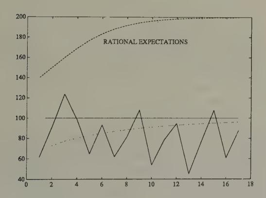
Figure 2:Path of inflation in Marimon and Sunder’s ‘Economy 7C’ (solid line). Also shown are one path conforming to the rational expectations dynamics converging to the higher stationary inflation rate of 200 percent, and a dotted line converging from below to the lower stationary inflation rate of 100 percent, which depicts a path associated with Marcet and Sargent’s least squares dynamics.
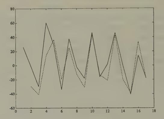
Figure 3:Solid line is record of sideliners’ mean prediction errors in Marimon and Sunder’s Economy 7C; dotted line is record of prediction error from least squares regressions of price on lagged price, using data up to time to make time forecasts.
Marimon and Sunder report many more experiments, and they analyze and interpret their results in interesting ways. Among other things, they perform a statistical analysis of the forecasting performance of the sideliners, and fit and test fixed-coefficient models of adaptive expectations à la Friedman and Cagan. This is part of an effort to learn about the details of the structure of adaptation that is propelling the experimental outcomes toward the low-inflation steady state.[8] [9]
An example in the spirit of Brock
In the Marimon-Sunder setting, least squares adaptation and the experiments both seem to select the ‘classical’ stationary equilibrium, which happens to be Pareto-superior to the other stationary equilibrium. As a warning not always to expect adaptation to select a Pareto-superior outcome, I offer the following example, composed by taking a special version of William Brock’s (1974) money-in-the-utility-function model of the demand for currency.[10]
An infinitely lived representative household maximizes
subject to the sequence of budget constraints,
and , given. Here is consumption of a single good, is a fixed endowment of the consumption good, is currency held from to , is the time price level, is the amount lent at a gross real rate of interest of . A government issues currency to finance a fixed level of expenditures , subject to the sequence of budget constraints , where is the supply of currency, and where in equilibrium .
Assume the restrictions on parameter values . Then this model has a unique stationary equilibrium, with , gross inflation rate determined by the value of that solves .[11] This stationary equilibrium value of has the ‘classical’ property that it is increasing in the value of the government deficit .
However, the model also has a continuum of nonstationary equilibria, indexed by initial price levels that are lower than the initial price level associated with the stationary equilibrium. In all of these equilibria, , so that these equilibria are characterized by deflation. These equilibria exist because the demand for currency induced by the preference ordering (8) is so elastic with respect to the rate of return on currency that there is room for a system of expectations in which the government can collect enough seigniorage to finance even while it pays out interest on its currency through deflation. These equilibria are definitely not ‘classical,’ because they imply that, within limits, higher values of are not associated with higher permanent values of inflation. An example of a nonstationary equilibrium is shown in Figure 4 and Figure 5, which starts from an initial rate of return on currency of unity. For this example, we set , , , . Notice how the rate of return on currency approaches , and how the equilibrium level of real balances explodes.
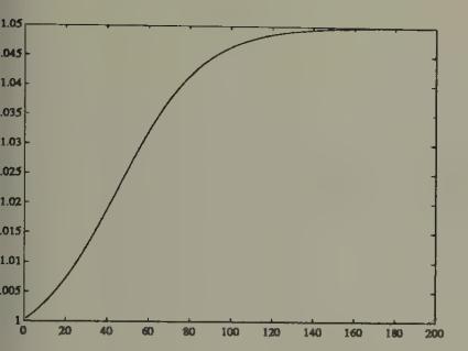
Figure 4:Time series of gross rate of return on currency (reciprocal of gross inflation rate) in Brock economy with , , , , under rational expectations dynamics.
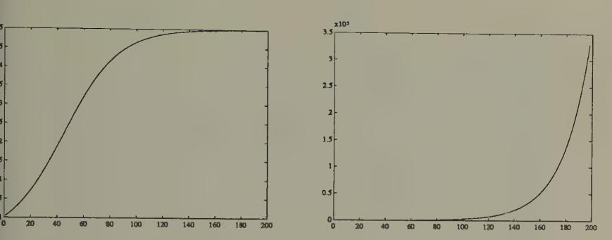
Figure 5:Time series of real value of currency in Brock economy under rational expectations dynamics.
This model shares with the overlapping-generations model the property that the ‘classical’ stationary equilibrium is unstable under the rational expectations dynamics. However, unlike the overlapping-generations model studied by Marimon and Sunder, the nonstationary rational expectations equilibria all Pareto-dominate the ‘classical’ stationary equilibrium.
What about the behavior of this model under ‘adaptive’ dynamics? If we were to use a version of the least squares learning mechanism studied by Marcet and Sargent (1989c), we would find that the ‘classical’ equilibrium is stable, while the nonstationary equilibria are not. Thus, this example shares with the overlapping-generations example the property that least squares dynamics selects a ‘classical’ stationary equilibrium. But the example also serves to warn us not to expect as a general rule that least squares dynamics will select a Pareto-superior equilibrium.[12]
Exchange rate experiments
The experiment
Jasmina Arifovic (1993) has performed an experiment with human subjects in an overlapping-generations environment with two currencies. The model which the experiment sought to implement was identical with the overlapping-generations economy studied by Marimon and Sunder, except that there were fixed supplies of two currencies, and , respectively, and young agents were given the opportunity to allocate their savings between the two currencies. Arifovic set the experiment up a little differently from Marimon and Sunder’s. She asked each young person to choose both a savings rate and a fraction allocating total savings between the two currencies. Let the savings rate for person be and the portion of the savings going to currency 1 be . Then the price levels at time were determined as described in Chapter 4, namely by
Also, Arifovic split the group of participants into two groups of equal size, one of which was young in odd periods, the other being young in even periods. Thus, unlike the situation in the Marimon-Sunder experiments, participants knew in advance when they would be born again. Arifovic also ended the experiments differently from Marimon and Sunder. In the final period, which was unknown beforehand to the participants, after the young people made their saving and portfolio decisions, she told the participants that this was the last period. It was known in advance that she would redeem money held by this last generation of young at a price level determined as the average of the price levels of the previous two periods.[13]
Exchange rate paths
Figure 6, Figure 7, and Figure 8 display exchange rate paths from three sessions of Arifovic’s experiments. The same set of subjects was used for each of the three sessions. Figure 9 displays the total saving rates of the young in experiment 1. For purposes of comparison, one can compute that in the rational expectations equilibrium the savings rate should be .
The exchange rate fluctuates within a range from 0.5 to 2. It does not settle down to a constant; if anything, the amplitude of the fluctuations grows between sessions 2 and 3. Figure 9 and Figure 10 display the savings rates for session 3.
Evidently, the simple least squares adaptive model used in Chapter 4 does a poor job of explaining these experimental data. But using a version of a genetic algorithm,[14] Arifovic has produced an economy with a population of adaptive agents that is capable of generating much exchange rate volatility. We now turn to her model.
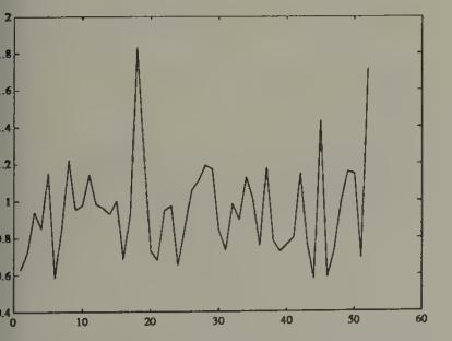
Figure 6:Exchange rates from Arifovic’s first session.
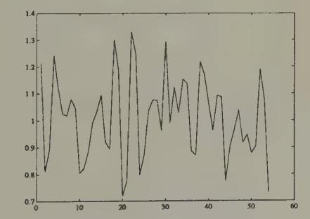
Figure 7:Exchange rates from Arifovic’s second session.
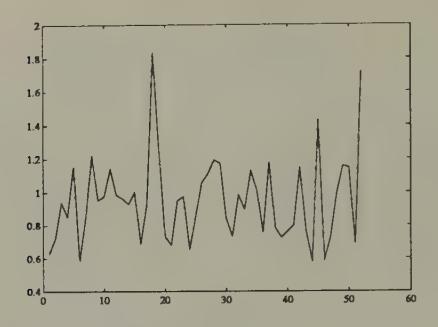
Figure 8:Exchange rates from Arifovic’s third session.
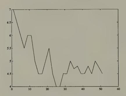
Figure 9:Saving rates for odd agents from Arifovic’s first session.
Figure 10:Saving rates for even agents from Arifovic’s first session.
A genetic algorithm economy
Arifovic studied a version of this economy using the genetic algorithm. The economy was inhabited by overlapping generations of two populations of agents of fixed sizes . A population of young agents consisted of a list of binary strings of length . The first 20 elements of a string were used to encode the saving decision parameter , and the second 10 were used to encode the portfolio division fraction . The ‘fitness’ of strings was evaluated according to the ex post value of the utility function (1), evaluated after the lifetime experience of the agent had been realized.[15]
Figure 11 through Figure 14 show parts of a record of exchange rates from the genetic economy.[16] The realized exchange rates are more variable than those found in Arifovic’s experiments. There are some quiescent periods for the exchange rate, as shown in parts of Figure 14, which covers observations 1801 through 1900, but they come to an end.
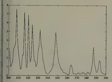
Figure 11:Exchange rate from genetic economy (observations 201--300).
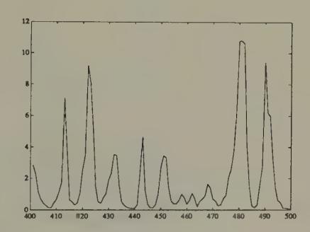
Figure 12:Exchange rate from genetic economy (observations 401--500).
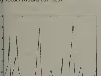
Figure 13:Exchange rate from genetic economy (observations 901--1000).
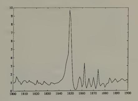
Figure 14:Exchange rate from genetic economy (observations 1801--1900).
Figure 15 shows the spectrum of a windsorized difference of the log of the exchange rate for observations 1000--2000. The spectrum is indicative of the first difference of a series whose level resembles a random walk, except that there is pronounced ‘mean reversion,’ as indicated by the dip in the spectrum at zero frequency.[17] The spectra of log differences of actual exchange rates for two typical hard currency countries for the post-1973 period resemble Figure 15, except they don’t have the dip at zero frequency.[18] Vis-à-vis the model of exchange rates with Newton-Raphson adapting agents, Arifovic’s genetic model generates much more ‘realistic’ exchange rate behavior.
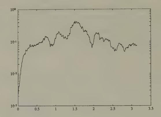
Figure 15:Spectrum of difference of logarithm of exchange rate for Arifovic’s genetic economy (observations 1000--2000). The spectrum indicates nearly random walk behavior for the log of the exchange rate, modified by the presence of mean reversion.
In addition to studying the stability of the two stationary equilibria under rational expectations and adaptive dynamics, Bruno and Fischer (1990) study how the existence of the ‘bad Laffer curve’ equilibrium can be precluded through choice of a monetary--fiscal policy operating rule.
The strict Pareto ranking of these equilibria depends on the absence of heterogeneity within a generation in this model. In versions of the model with heterogeneity within generations (e.g., the borrowers and lenders of Wallace 1980), the equilibria are not Pareto-comparable. See Sargent and Wallace (1982).
George Evans and Seppo Honkapohja (1992c) study the stability of ‘sunspot equilibria’ under adaptive least squares learning algorithms. In particular, they study the stability of sunspot equilibria that can be constructed near both stationary and periodic fundamental or non-sunspot equilibria. They show that the stability under adaptive learning of sunspot equilibria near fundamental equilibria is inherited from the stability under adaptive learning of the fundamental equilibria out of which they are constructed. For example, they show that the stability under learning of two-state sunspot equilibria that are constructed near period 2 fundamental equilibria requires stability under learning of the period 2 equilibrium; and that stability under learning of two-state sunspot equilibria that are constructed out of two stationary (i.e. period 1) fundamental equilibria requires stability under learning of both of the fundamental equilibria.
See Bullard and Duffy (1993) for a warning not to overgeneralize from this result.
Marimon and Sunder show that equilibria outcomes of the overlapping-generations economy are among the equilibria of the game that their experiment defines.
In forming their supply schedules, the subjects are implicitly forecasting the price level at time , because their payoff depends on it.
These are ‘honest’ errors for the least squares forecaster, because the least squares regression coefficient used to make time forecasts uses the observations on the experimental prices only through time .
Can we expect laboratory experiments with paid students to increase our understanding of how actual monetary economies would operate? Even if the experimenter succeeds in inducing the preferences that he wants, the behavior of a randomly selected population of students might very well differ systematically from the self-selected and performance-censored sample of traders operating in foreign exchange markets. See Friedman and Sunder (1992) for an extensive analysis of experimental methods.
If they were available, econometric studies of econometrically identifiable models with multiple equilibria would provide an alternative to using experimental economies as a benchmark with which to compare the equilibria selected by adaptive algorithms. However, I know of few such econometric studies. One study is by Selahattin Imrohoroglu (1993), who fits a rational expectations version of the same model used by Marimon and Sunder to data from the German hyperinflation. Imrohoroglu estimates parameters that index the multiplicity of rational expectations equilibria. Despite the multiplicity of equilibria, his model is econometrically overidentified, which permits him to estimate which of the continuum of equilibria best describes the sample data, as measured by a Gaussian likelihood function. His estimates are consistent with the hypothesis that the observations come from an equilibrium with neither stochastic nor nonstochastic bubbles, but nevertheless are not consistent with the data having been generated from the low-inflation equilibrium. His estimated equilibrium is sliding along the bad side of the Laffer curve, toward the high stationary inflation rate. Thus, these results are inconsistent with the hypothesis that the data were generated from the equilibrium selected by the adaptive dynamics. Imrohoroglu explains how this outcome emerges because the likelihood function is insisting on activating or ‘mixing’ both of the system’s two endogenous roots (the low and high stationary nonstochastic equilibrium inflation rates) in order to match the salient lower frequency features of the data, namely, decreasing real balances and increasing inflation rates.
This example was shown to me by Benjamin Bental.
Namely, .
See Moore (1993) for an application of least squares learning to select between stationary rational expectations equilibria in a model of Howitt and McAfee (1988). Moore finds that the low-employment equilibrium is not stable under least squares learning but that the high employment equilibrium can be.
Parameter values were , , , .
Arifovic added what she called an election operator to the sequence of operators used by Holland to define the genetic algorithm. The election operator tests the ‘children’ of a pair of parents to see whether they are fitter as judged by last period’s data fed into the performance criterion. If the children are fitter by that measure, they replace their parents. Otherwise, the parents live on and the children are not born.
Arifovic carried along two populations of odd and even agents, letting each population choose every other period, for the reasons explained in the Chapter 4 discussion of the least squares adaptive exchange rate model.
Arifovic generated 20,000 observations, and we show pieces of the first 2000.
‘Windsorizing’ is achieved by naming two bounds with , and replacing every observation less than with and every observation greater than with . Where data are suspected of having distributions with infinite variances, windsorizing is a technique devised to assure that spectral densities are well-defined.
The economic environment in which Arifovic’s genetic algorithms operate does not contain any of the classic forces for low-frequency divergences in exchange rates.