7. Applications
I conclude this essay by pointing to some promising applications of the methods that we have surveyed, and also to some limitations.
Evolutionary programming
We have studied several examples in which systems of adaptive agents eventually find their way to a rational expectations equilibrium, and we know from results in the literature that there is a big class of other models where convergence will also occur. The examples in this book have all been ones that are simple enough for us to compute equilibria beforehand, then watch how fast and to which equilibrium the adaptive system converged. The idea of evolutionary programming is to use the equilibrium-finding tendency of collections of adapting agents to compute equilibria for us.[1]
Kiyotaki--Wright search models
Adaptive methods have been used to discover equilibria of enriched versions of Kiyotaki and Wright’s (1989) search model of monies. Kiyotaki and Wright’s original model is an infinitely repeated ‘Wicksell triangle’ economy. There are continua[2] of three types of household. Each type of household produces its own type of good, but likes to consume only the good of the type of consumer to its ‘right’ along the triangle. Goods are indivisible, and each consumer can store only one unit of any good at a time, with costs of storage differing among goods. Each period, a consumer is pairwise randomly matched with one of the other consumers whom he/she expects never to meet again. Kiyotaki and Wright’s economy is set up to preclude coincidence of wants, and to require that trade be mediated via a ‘medium of exchange,’ a good that some of the traders occasionally take and hold in the expectation that they can trade it later for the good that they want to consume. Kiyotaki and Wright formulate Nash equilibria of this economy, and describe a method for stationary equilibria. A stationary equilibrium for Kiyotaki and Wright’s model is a collection of trading strategies for each type, and a set of probabilities of meetings between households storing different types of goods.
Marimon, McGrattan, and Sargent (1990) put collections of Holland classifier systems inside two of Kiyotaki and Wright’s economic environments[3] and watched them converge to an equilibrium. Litterman and Knez (1989) put three populations determined by a genetic algorithm into a Kiyotaki--Wright environment, and these also found their way to an equilibrium. Encouraged by these results, Marimon, McGrattan, and Sargent created a pentagonal version of Kiyotaki and Wright’s environment, with five types of households and goods, and populated it with five types of classifier systems. This system settled down to a collection of trading strategies and probabilities that could then be verified to be an equilibrium.
The idea of evolutionary programming is to use adaptive algorithms to inspire a ‘guess,’ then to use the ‘guess and verify’ method of solving the functional equations that determine an equilibrium. Randall Wright (1993) has used this method to compute the equilibrium of a version of the original Kiyotaki--Wright model in which the fractions of different types of agents are endogenous.[4] Instead of having equal measures of the three types of households, he let there be fractions that are chosen to make the payoffs to the three types of agents equal. He set up an evolutionary system to find such an equilibrium, whose equilibrium conditions are all of the equilibrium conditions of the original Kiyotaki--Wright model, plus the restriction that payoffs are equal across types. For fixed vector , Wright used the methods of Kiyotaki and Wright to compute a ‘fixed-’ equilibrium, then calculated payoffs to the different types. Then he let the fraction of the types evolve, according to a version of the ‘reproduction operator’ within the genetic algorithm. The share vector eventually evolved to a point at which payoffs were equalized. Such a point is automatically an equilibrium, because by construction it builds in all of the equilibrium conditions.[5]
Wright used evolutionary methods not because he was interested in the evolutionary dynamics, but as a method of finding an equilibrium. From this standpoint, it is interesting how Wright divided the work of equilibrium computation between himself and the adaptive agents. For each vector along the evolutionary process, Wright computed a fixed- equilibrium, and computed the expected value of the infinite-horizon payoff function for all agents at that equilibrium. He then ‘told’ the evolutionary process those theoretical payoffs, and let the fraction of agents adapt to them. Notice how this division of labor makes the process hard to interpret in terms of ‘real-time dynamics’ because Wright is giving agents information about payoffs that they could acquire only by experiencing very long histories within fixed- regimes. But from the viewpoint of Wright’s interest in equilibrium computation, the process’s lack of credibility as real-time dynamics is irrelevant.
How adaptive agents teach smart economists
In using systems of adaptive agents to generate a ‘guess,’ we are counting on the tendency of these systems of adaptive agents, as plodding as they are, eventually to find their ways to equilibria that we economists (who, after all, made up the environment!) have difficulty finding, despite all of our advantages relative to those agents in terms of knowledge about the way the whole system is put together.
There is nothing magic or new going on here. The adaptive agents are ‘teaching’ the economist in the same sense that any numerical algorithm for solving nonlinear equations ‘teaches’ a mathematician. When these agents can ‘teach’ us something, it is because we designed them to do so.
Solving recurrent single-agent problems
There exist a number of examples in which an artificial device has been trained to learn a good strategy to apply within an environment that is complicated enough to challenge an expert in decision theory. The method is simple: put the artificial device within a computer representation of the environment, and use simulations to train it.
An iterated prisoner’s dilemma
Robert Axelrod (1987) used the genetic algorithm to train a population to play against the computer programs that had been submitted by participants in his round-robin computer tournament to play the iterated prisoners’ dilemma. He encoded strategies as binary strings of length 70, with the last 64 of the bits used to dictate play following each of the 64 possible histories of play in the history of the three previous moves,[6] and the first six bits being used to encode initial play. The algorithm produced a strategy that would have won the tournament, and in particular would have outplayed the ‘tit-for-tat’ strategy that won the tournament.[7] Interestingly enough, the winning genetic strategy behaved much like ‘tit-for-tat’ when confronted with non-tit-for-tat strategies, but sufficiently tougher against tit-for-tat that it could take advantage of it.
A double oral auction
Rust, Palmer, and Miller (1992) set up a computer tournament to play the double oral auction. Participants submitted programs encoding their strategies, then the computer ran auctions, and kept accounts of earnings. Participants received monetary rewards in proportion to those earnings.
The winning strategy in the tournament was submitted by a graduate student at the University of Minnesota, Todd Kaplan. Kaplan’s strategy abstains from making bids or offers, but waits and watches other people make bids and offers, then ‘steals the trade’ when bids and offers get close enough together. A market composed mostly of traders like Kaplan would have behaved badly, and not to Kaplan’s benefit, but enough other participants submitted strategies with aggressive bid and offer components that Kaplan prospered.
Rust, Palmer, and Miller (1992) went on to use neural networks to encode a class of potential strategies, then to train them by allowing them to compete against each other and a collection of other strategies for very long simulations. In choosing a class of neural nets, Rust, Palmer, and Miller were in effect choosing the domain of a nonlinear function (i.e., what information the strategy could potentially condition on) and the class of nonlinear decision rules that could potentially be learned (controlled by the number of ‘hidden units’). Rust, Palmer, and Miller used a genetic algorithm to estimate or train the neural nets. There were neural nets for both ‘buyers’ and ‘sellers.’
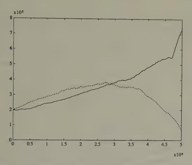
Figure 1:Evolution of capital for two ‘sellers’ in computer tournament of double oral auction. The solid line is the cumulated earnings of a ‘Kaplan’ seller; the dotted line is the cumulated earnings of what for a long time seemed to be the best neural network seller.
During the early part of one of Rust, Palmer, and Miller’s simulations with 52 sellers and buyers, with some of them being neural net traders, one of the neural network sellers does better than a Kaplan seller. Figure 1 records the cumulative earnings for the best neural network seller and Kaplan. The superiority of the neural network over Kaplan eventually vanishes later in the simulation. Thus, after a very long training session, Rust, Palmer, and Miller failed to produce a neural network that would have done better than Kaplan’s. These results show the difficulty confronted by a relatively unprompted artificial device in discovering rules that defeat the simple but shrewd strategy devised by the human Kaplan.[8]
Forecasting the exchange rate
Estimates of vector autoregressions for exchange rates for leading ‘hard currencies’ over the post-1973 period of floating rates have revealed that it is difficult to find a linear model that outforecasts a simple random walk (or ‘no change’) model. Researchers have used sophisticated methods for detecting nonlinearities in exchange rates, and found evidence for their presence. Encouraged by these findings, Diebold and Nason (1990) and Kuan and Liu (1991) have sought to find particular nonlinear forecasting functions that can be estimated with sufficient precision to produce better forecasts than do linear models.[9]
Kuan and Liu’s method was to specify and estimate a neural network as a device for estimating a potentially nonlinear autoregression. Kuan and Liu did not have Rust, Palmer, and Miller’s luxury of training their network on arbitrarily long simulations, but had to train it on the available time series from the post-1973 period. For this reason, they had to face issues of overfitting. They used the Rissanen complexity criterion to arrive at models for a collection of exchange rates, which they then used to produce and evaluate ‘honest forecasts.’
Let be the exchange rate, and . The simplest model that Kuan and Liu fitted was of the form
where is a forecasting error, and is determined by a neural network of the form
where is the sigmoid function . Kuan and Liu fitted their models to daily closing prices from 1987 to 1991 for five countries, then used the models to forecast out of sample.[10] Figure 2 and Figure 3 show the nonlinear function estimated by Kuan and Liu for the yen-dollar exchange rate.[11] We use two scales, to supply a magnifying glass for spotting the nonlinearity that the procedure has detected. The figures show how the neural network has managed to detect only a minuscule departure from the ‘martingale’ model (), and how in this case the autoregression is linear to a very good approximation.
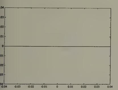
Figure 2:Estimated neural net function mapping change in log of yen-dollar exchange rate today into prediction for change in log of yen-dollar exchange rate tomorrow. The neural net essentially estimates a ‘martingale difference’ model for the log exchange rate.
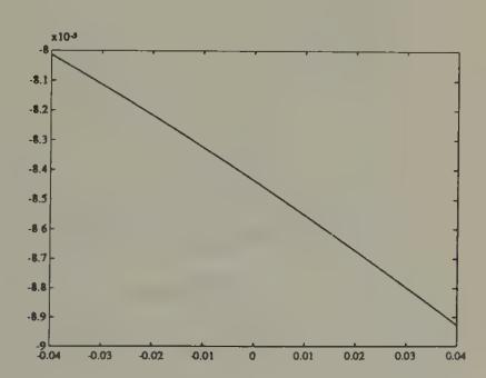
Figure 3:Estimated neural net for forecasting yen-dollar exchange rate---finer scale on coordinate axis. Notice the very mild nonlinearity.
It is interesting that these techniques fail to find substantial deviations from linearity that would be useful for predicting in this particular context.[12] Undoubtedly, application of such techniques in other contexts will detect deviations from linearity that are exploitable for forecasting.
A model of policy-makers’ learning
Within the rational expectations literature in macroeconomics, there is a strand that interprets the post-World War II covariation of unemployment and inflation in the United States as reflecting the interaction between a private sector whose behavior was summarized by an expectational Phillips curve embodying both rational expectations and the natural unemployment rate hypothesis, and a government whose behavior at least for a time was driven by the erroneous belief that there was an exploitable Phillips curve.[13] The story is that Phillips curves were estimated with data through the 1960s; that these indicated a tradeoff between inflation and unemployment that the government believed to have been exploitable; and that government policy-makers tried to lower unemployment in the late 1960s and early 1970s by managing aggregate demand to generate inflation. The story asserts that the consequence of these actions was to cause the Phillips curve to shift up adversely, leading to higher inflation with no benefits in terms of lower unemployment on average.
However, this story has been disputed by various fitters of 1960s style Phillips curves, who argued that their econometric procedures were adaptive, and were able to detect the adverse shift in the Phillips curve swiftly enough to give sound policy advice.
Christopher Sims (1988) described an econometric specification capable of representing both the ‘natural rate’ story, with its combination of a rational private sector and an irrational government, and the alternative story that traditional Phillips curve fitters caught on to what was happening soon enough to give the government timely advice. Sims wanted a manageable model that could formalize the informal procedures that Phillips curve fitters in practice used to protect themselves against some of the effects of specification errors. He formulated a model of boundedly rational macroeconomic policy-makers who use a plausible econometric strategy for learning about a Phillips curve tradeoff. The model can have multiple types of equilibria, one of which displays the feature that introducing uncertainty into the government’s (erroneous) model can sometimes lead the system toward an approximately optimal outcome. Heetaik Chung (1990) estimated a version of the model for post-World War II time series from the United States. This is the only econometrically serious macroeconomic implementation of bounded rationality of which I know.
The model is an extended version of Kydland and Prescott’s (1977) Phillips curve example. The rate of inflation is decomposed as
where is the rate of inflation at time , is the expected rate of inflation as of time (i.e., , where is the public’s time information), and is the public’s error in forecasting inflation. The government can control but not the forecast error , which is assumed to be orthogonal to information available to the public at dates earlier than . Unknown to the government, there is truly a natural-rate Phillips curve of the form
where , is the natural rate of unemployment, and is a covariance stationary stochastic process that is orthogonal to . Only the unexpected part of inflation influences the unemployment rate, but the government does not (at least in the beginning) realize this.
At time , policy-makers (incorrectly) estimate that the Phillips curve is of the (non-expectational) form
where are the government’s time estimates of parameters of the Phillips curve, and is a statistical residual, which the government believes to be serially uncorrelated. The policy-maker sets myopically to maximize
subject to the perceived constraints
Therefore, the government’s decision rule is
Constant coefficient beliefs
As a benchmark, Sims and Chung first formalize a least squares learning process that in the limit converges to Kydland and Prescott’s ‘consistent equilibrium.’ The government believes a version of model (5) in which (apart from estimation error) the coefficients , are constant over time. Each period the government updates its estimates using ordinary least squares, and then implements (8) using its latest parameter estimates. This practice generates a ‘self-referential’ system because the actual relation between inflation and unemployment depends on the government’s false perception of the relation (5) and the action (8) that it takes on the basis of that perception. This produces a least-squares learning process that converges to Kydland and Prescott’s consistent equilibrium in which the coefficient estimates eventually satisfy
Consequently, converges to , with . This outcome gives lower utility to the government than it could have attained if it had understood that the true Phillips curve was (4). If the government had known the true Phillips curve, it would have attained the same unemployment rate it eventually got, but with , which evidently would have been better. This outcome comes from Kydland and Prescott’s ‘optimal policy.’
Random coefficient beliefs
Sims and Chung modified the model in a way designed to attribute model uncertainty to the government. They assumed that the government’s beliefs are described by a random-coefficients version of model (5) in which the government suspects that the ‘true coefficients’ are taking a random walk:
where is a Gaussian white noise with and being diagonal with . The parameters in index the government’s degree of confidence in the constant-coefficient, linear specification.
Sims and Chung assumed that the government applies the Kalman filter to estimate the random coefficients model comprised by (5) and (10), given values of the parameters ; and that the government continues to make policy on the basis of the myopic rule (8).[14] Sims showed how this model can exhibit two types of behavior. First, some histories of the model look like (noisy) versions of the model in which the government has constant-coefficient beliefs, and converge to the vicinity of a consistent equilibrium. However, other histories converge to a stochastic process that spends most of its time near the optimal zero-inflation outcome. Along these paths, because of its willingness to entertain random coefficients in the model it is fitting, the government is rather quickly learning (without putting the economy through a big inflation) that the Phillips curve tradeoff is poor, which dampens its enthusiasm for exploiting it. Which type of path emerges depends partly on the parameter values (especially the parameters indexing the government’s certainty about the form of the model). Notice how these two types of paths represent formalizations of the story and the counter-story described at the beginning of this section.
Econometric implementation
Chung specified and estimated an enlarged version of this model using post-war US time series. He extended the specifications of the true and government-perceived Phillips curve (4) and (5), respectively, to permit lag structures more capable of matching the data, partly by explicitly modelling serial correlation structures of disturbance processes. As the econometrically free parameters he took and the variances of the other shocks in the model, where is the prior mean of the vector, used to initiate the government’s Kalman filter. He wrote down a Gaussian quasi-likelihood function conditioned on a data record , and maximized it with respect to the free parameters. This procedure permitted Chung to estimate a model of the government’s learning process. A product of Chung’s estimation is a history of the government’s beliefs and its decision rules (8).
Thus, Chung estimated and discussed the altered state of the government’s perceptions about the Phillips curve, and a time-varying decision rule of a form extending (8) during the post-war period, and advanced intriguing interpretations about how his estimates match up with informal non-econometric interpretations of how beliefs about the Phillips curve impinged on government macroeconomic decision-making.
In addition to its interesting substance, the work of Chung and Sims is important for demonstrating the practical possibility of econometrically implementing a model in which the econometrician is imputing the application of non-trivial econometrics procedures to one or more of the agents within the estimated model. If bounded rationality is to be put to work in macroeconomics, this is only the first of this type of work that we shall see.
Limitations
Prompting
Rational expectations imposes a specific kind of consistency condition on an economic model. The idea of bounded rationality is perhaps best defined by what it is not (rational expectations), a definition that captures the malleability of bounded rationality as a principle of model building. Even after we have adopted a particular class of algorithms to represent the adaptive behavior of a collection of agents, we have seen repeatedly that we face innumerable decisions about how to represent decision-making processes and the ways that they are updated.
As model builders, we decide how much agents know in advance, what they don’t know and must learn about, and the particular methods they have to use to learn.[15] Do they know their utility and profit functions, or must they learn about them? Do they know calculus and dynamic programming, or must they only use ‘trial and error’ methods? Do they learn only from their own past experiences or from those of others?[16] To what class of approximating functions do we restrict them in specifying what they learn about?
Contributions to the bounded rationality literature have taken many different stands on these issues. The example of Bray in Chapter 5, and some of the examples described by Marcet and Sargent (1989a, 1989b), give the artificial agents a lot of ‘prompting.’ In Bray’s model, agents know the correct supply curve, and must only estimate the correct conditional expectation to plug into it.[17] Some of Marcet and Sargent’s examples are in the adaptive control tradition of assuming that agents use dynamic programming to compute an optimal decision rule, that they know the parameters of their return function and the parametric form of the transition function, but that they lack knowledge of the parameters of the transition function. So each period, these agents are supposed to use Litterman--Sims-style econometric methods to update an estimated vector autoregressive representation of the unknown pieces of their transition equation, then to solve their dynamic programming problem given their most recent estimates of the transition law.[18]
The classifier systems that live in Marimon, McGrattan, and Sargent’s (1990) version of Kiyotaki--Wright models receive much less prompting than the agents of Bray and Marcet and Sargent, but they still get a lot. Marimon, McGrattan, and Sargent’s agents are not told their utility functions; they recognize utility only when they experience it. They are ignorant of dynamic programming, and can come to appreciate the consequences of sequences of actions only by trying them out, then experiencing the utility of their consequences. Still, they are prompted. They are told when to choose and what information to use. The size and structure of their classifier systems, including the details of the accounting system, and the generalization and specialization operators, are chosen for them by Marimon, McGrattan, and Sargent, who obviously had an eye on specifying these things so that the artificial agents would have a good chance to learn to play the Kiyotaki--Wright equilibrium.[19]
Simplicity
All of the examples that we have studied are very simple in terms of the econometric problems with which we have confronted our artificial agents. We have given our agents the task of learning either a time-invariant decision rule or a collection of conditional expectations. It is easy to imagine settings in which more complicated tasks would be assigned to the agents. Useful ways of complicating these tasks can be found by following the topics treated in a modern econometrics course. For example, we might make our agents learn about the parameters of an econometric structure using the methods of classical simultaneous equations or rational expectations econometrics. The point of these methods is not to learn about a single decision rule or probability distribution but about a mapping from parameters characterizing policy regimes to functions or probability distributions.[20]
Bounded rationality and the econometricians
Bounded rationality is a movement to make model agents behave more like econometricians. Despite the compliment thereby paid to their kind, macroeconometricians have shown very little interest in applying models of bounded rationality to data. Within the economics profession, the impulse to build models populated by econometricians has come primarily from theorists with different things on their minds from most econometricians.
Applied time series econometricians have largely ignored the bounded rationality program because they accept a canon embodied in Lucas’s warning to ‘beware of theorists bearing free parameters.’[21] Within a specific economic model, an econometric consequence of replacing rational agents with boundedly rational ones is to add a number of parameters describing their beliefs and the motion of their beliefs.[22] For example, relative to a rational expectations model, count the number of additional free parameters that would be associated with implementing the model of Bray that appeared in Chapter 5. For a single-agent version of the model, one would add the parameter characterizing initial beliefs, and a parameter initiating the gain sequence. One might want to add other parameters characterizing the shape of the sequence. These parameters would be a nuisance to estimate for technical reasons associated with the fact that, because of Bray’s result about convergence to rational expectations, these parameters only influence transient dynamics: the asymptotic distribution of contains no information about these parameters. Multiple-agent versions of Bray’s model would have additional parameters, and so would any of the larger example models that we have studied.
Transition dynamics
Because of the preceding limitations, the literature on adaptive decision processes seems to me to fall far short of providing a secure foundation for a good theory of real-time transition dynamics. There are problems of arbitrariness and the need for prompting, with a concomitant sensitivity of outcomes to details of adaptive algorithms. There is the extreme simplicity of the learning tasks typically assigned in the models compared even with the econometric learning tasks assigned in econometric classes, to say nothing of those implicitly being resolved by firms and households. In particular, the environments into which we have cast our adaptive agents seem much more stable and hospitable than the real-life situations for which we would want transition dynamics. On the purely technical side, there is the shortage of results on rates of convergence, and the need severely to restrict the distribution of agents’ beliefs in order to get tractable models. And most important, and surely partly a consequence of the earlier limitations, applied econometricians have supplied us with almost no evidence about how adaptive models might work empirically.
It would not be wise or fair to end this essay by dwelling on the failure of adaptive methods so far to have ‘hit a home run’ by giving us a good theory of transition dynamics. The problem of transition dynamics is difficult and long-standing. So maybe it should count as a single, or at least a sacrifice fly, that these methods have sharpened our appreciation of the problem. And adaptive methods have given us other hits.
Successes and promises
I finish this essay by listing the things about adaptive algorithms in macroeconomics that I think will become more and more useful. Despite my reservations about them as theories of real-time dynamics, I like adaptive algorithms as devices for selecting equilibria.[23] Evolutionary programming is a valuable tool for computing equilibria, and is likely to be applied often. Econometricians are likely to continue to find useful devices in the literatures on adaptation. Econometricians are now using genetic algorithms and stochastic Gauss-Newton procedures, even if the agents in the models that they are estimating are not.
We have already seen that Marcet’s method of parameterized expectations has many aspects of a learning or adaptation algorithm.
The continua are of equal measure.
Kiyotaki and Wright described two environments, model A and model B, that differed in the arrangement of preferences for goods within the Wicksell triangle.
Wright used this model to capture some responses that are shut down by Kiyotaki and Wright’s assumption of fixed and equal shares, which affects the payoffs to types in ways that provoke no response in the original model.
Matsuyama, Kiyotaki, and Matsui (1992) used evolutionary methods to determine the stability of equilibria of an extension of the Kiyotaki--Wright model in which multiple currencies can emerge.
There are four possible combinations of moves each time the one-period game is played, meaning that there are 43 possible histories of length 3.
The genetic algorithm had a big advantage over the participants in the tournament because it got to practice against them, while they could only guess what opponents’ strategies would be.
Rust, Palmer, and Miller (1992) make interesting observations on the extent to which simulations of markets populated by groups of neural networks look like those populated by human players of the double oral auction.
Diebold and Nason (1990) used nonparametric methods to see if nonlinearities that have been detected in post-Bretton Woods exchange rates could be exploited to generate better point predictions than are yielded by a linear model. They did not find them.
Kuan and Liu used two types of estimators. The first was an ‘on-line’ algorithm of the kind described in Chapter 4. The second was an ‘off-line’ version of nonlinear least squares. I report the results for nonlinear least squares. Kuan and Liu discuss how the ‘on-line’ algorithm can be used to make several passes through the data, with the final estimates from the last pass being used as the initial estimates from the next pass.
Canova (1993) uses a Bayesian vector autoregression with time-varying coefficients to represent and estimate a model of exchange rates with particular types of nonlinearities. See his paper for a discussion of the types of nonlinearities that seem to infest exchange rate data.
Kuan and Liu also fitted what amount to higher-order nonlinear univariate autoregressive models for exchange rate log differences.
For a discussion of some of the issues, see Lucas (1981, pp. 221, 283).
The Kalman filter can be formulated as a stochastic approximation algorithm. For example, see Ljung, Pflug, and Walk (1992, pp. 99--100).
We decide how they are ‘hard-wired.’
Ellison and Fudenberg (1992) study evolutionary systems in which people condition their choices on how a fraction of agents in the population have acted in the past.
In games of fictitious play, players play best responses to estimates of probability distributions formed from histograms of past play. Though the setting is different, the spirit is the same as Bray’s.
This scheme is irrational because agents are ignoring the consequences of estimation uncertainty when solving their dynamic programming problem.
See Marimon and McGrattan (1993) for a critical review of adaptive algorithms within the context of games. Also see Kreps (1990).
See Hurwicz (1946) for a brief discussion.
John Taylor (1975) and Christopher Sims (1988) have used systems with adaptive agents to make interesting theoretical points. We have described how Chung (1990) implemented such a model empirically.
The model of Chung (1990) described above illustrates these points in a simple context, while also demonstrating that such an analysis is feasible.
I know that it is inconsistent to doubt the real-time dynamics but keep the equilibria selected by them. I confess that my affection for the selection performed in the monetary models described in Chapter 6 is partly driven by my prior conviction that the selected equilibria seem sensible to me.