5. Pandas#
Anaconda-യിൽ ഉള്ളവ കൂടാതെ, ഈ lecture-ന് താഴെ പറയുന്ന libraries-ഉം ആവശ്യമായിവരുന്നു:
!pip install --upgrade wbgapi
!pip install --upgrade yfinance
5.1. Overview#
Pandas എന്നത്, Python-നായുള്ള വേഗതയേറിയതും കാര്യക്ഷമവുമായ data analysis tools-ന്റെ ഒരു package ആണ്.
data science, machine learning തുടങ്ങിയ മേഖലകളുടെ വളർച്ചയ്ക്കൊപ്പം, ഈ package-ന്റെ popularity അടുത്ത വർഷങ്ങളിൽ വളരെയധികം ഉയർന്നിട്ടുണ്ട്.
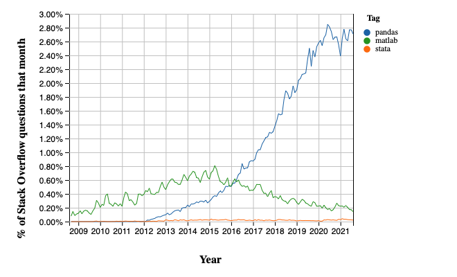
Stack Overflow Trends-ന്റെ സഹായത്തോടെ, Matlab-ഉം, STATA-ഉം ആയി താരതമ്യം ചെയ്യുന്ന ഒരു popularity comparison കാലക്രമേണ താഴെ കാണാം:
NumPy, അടിസ്ഥാന array data type-ഉം core array operations-ഉം നൽകുന്നത് പോലെ, pandas:
data-യുമായി പ്രവർത്തിക്കാനുള്ള fundamental structures define ചെയ്യുന്നു, കൂടാതെ
താഴെപ്പറയുന്ന operations-നെ സഹായിക്കുന്ന methods-ഉം അവയ്ക്ക് നൽകുന്നു:
data read ചെയ്യൽ
indices adjust ചെയ്യൽ
dates-ഉം time series-ഉം ആയി പ്രവർത്തിക്കൽ
sorting, grouping, re-ordering, പൊതുവായ data munging [1]
missing values കൈകാര്യം ചെയ്യൽ, etc., etc.
കൂടുതൽ sophisticated ആയ statistical functionality, pandas-ന് മുകളിൽ build ചെയ്തിരിക്കുന്ന statsmodels, scikit-learn പോലുള്ള മറ്റ് packages-ന് വിട്ടുകൊടുത്തിരിക്കുന്നു.
ഈ lecture pandas-നെക്കുറിച്ചുള്ള ഒരു basic introduction നൽകുന്നു.
ഈ lecture-ൽ ഉടനീളം, താഴെ പറയുന്ന imports നടന്നിട്ടുണ്ട് എന്ന് നമുക്ക് കരുതാം:
import pandas as pd
import numpy as np
import matplotlib.pyplot as plt
import requests
pandas define ചെയ്യുന്ന രണ്ട് പ്രധാന data types ആണ് Series-ഉം, DataFrame-ഉം.
Series-നെ data-യുടെ ഒരു "column" ആയി കരുതാം, ഉദാഹരണത്തിന് ഒരു single variable-ന്റെ observations-ന്റെ ഒരു collection.
DataFrame എന്നത്, ബന്ധപ്പെട്ട data columns സൂക്ഷിക്കാനുള്ള ഒരു two-dimensional object ആണ്.
5.2. Series#
നമുക്ക് Series-ഇൽ നിന്നും തുടങ്ങാം.
നാല് random observations-ന്റെ ഒരു series create ചെയ്തുകൊണ്ട് നമുക്ക് തുടങ്ങാം:
rng = np.random.default_rng()
s = pd.Series(rng.standard_normal(4), name='daily returns')
s
0    0.429189
1   -0.154323
2    0.581238
3   -3.216505
Name: daily returns, dtype: float64
ഇവിടെ 0, 1, 2, 3 എന്നീ indices, list ചെയ്തിരിക്കുന്ന നാല് companies-നെ index ചെയ്യുന്നു എന്നും, values അവയുടെ shares-ന്റെ daily returns ആണെന്നും നിങ്ങൾക്ക് സങ്കൽപ്പിക്കാം.
Pandas-ന്റെ Series, NumPy arrays-ന് മുകളിലാണ് build ചെയ്തിരിക്കുന്നത്, അതിനാൽ സമാനമായ പല operations-ഉം ഇത് support ചെയ്യുന്നു:
s * 100
0     42.918916
1    -15.432264
2     58.123845
3   -321.650516
Name: daily returns, dtype: float64
np.abs(s)
0    0.429189
1    0.154323
2    0.581238
3    3.216505
Name: daily returns, dtype: float64
എന്നാൽ Series, NumPy arrays-നേക്കാൾ കൂടുതൽ നൽകുന്നു.
Statistically oriented ആയ കുറച്ച് additional methods-ഉള്ളതിന് പുറമേ:
s.describe()
count    4.000000
mean    -0.590100
std      1.779409
min     -3.216505
25%     -0.919868
50%      0.137433
75%      0.467201
max      0.581238
Name: daily returns, dtype: float64
അവയുടെ indices കൂടുതൽ flexible ആണ്:
s.index = ['AMZN', 'AAPL', 'MSFT', 'GOOG']
s
AMZN    0.429189
AAPL   -0.154323
MSFT    0.581238
GOOG   -3.216505
Name: daily returns, dtype: float64
ഇങ്ങനെ നോക്കുമ്പോൾ, Series, വേഗതയേറിയതും കാര്യക്ഷമവുമായ Python dictionaries പോലെയാണ് (dictionary-യിലെ items എല്ലാം ഒരേ type-ൽ ആയിരിക്കണം എന്ന നിബന്ധനയോടെ --- ഇവിടെ floats).
വാസ്തവത്തിൽ, Python dictionaries-ന്റെ അതേ syntax തന്നെ നിങ്ങൾക്ക് ഇവിടെയും ഉപയോഗിക്കാം:
s['AMZN']
np.float64(0.4291891606826992)
s['AMZN'] = 0
s
AMZN    0.000000
AAPL   -0.154323
MSFT    0.581238
GOOG   -3.216505
Name: daily returns, dtype: float64
'AAPL' in s
True
5.3. DataFrames#
Series എന്നത് data-യുടെ ഒരു single column ആണെങ്കിൽ, DataFrame എന്നത് ഓരോ variable-ഇനും ഓരോ column ഉള്ള പല columns ആണ്.
അടിസ്ഥാനപരമായി, pandas-ലെ ഒരു DataFrame, ഒരു (highly optimized) Excel spreadsheet-ന് സമാനമാണ്.
അതിനാൽ, rows-ഇലേക്കും columns-ഇലേക്കും സ്വാഭാവികമായി organize ചെയ്യപ്പെട്ട data represent ചെയ്യാനും analyze ചെയ്യാനും, individual rows-ഇനും individual columns-ഇനും descriptive indexes ഉള്ളതോടെ, ഇത് ഒരു powerful tool ആണ്.
Penn World Tables-ൽ നിന്നും എടുത്ത test_pwt.csv എന്ന CSV file-ൽ നിന്നും data read ചെയ്യുന്ന ഒരു example നമുക്ക് നോക്കാം.
ഈ dataset-ൽ താഴെ പറയുന്ന indicators അടങ്ങിയിരിക്കുന്നു:
Variable Name |
Description |
|---|---|
POP |
Population (in thousands) |
XRAT |
Exchange Rate to US Dollar |
tcgdp |
Total PPP Converted GDP (in million international dollar) |
cc |
Consumption Share of PPP Converted GDP Per Capita (%) |
cg |
Government Consumption Share of PPP Converted GDP Per Capita (%) |
pandas-ന്റെ read_csv എന്ന function ഉപയോഗിച്ച്, ഒരു URL-ൽ നിന്നും നമുക്ക് ഇത് read ചെയ്യാം.
df = pd.read_csv('https://github.com/QuantEcon/data-lectures/raw/main/lectures/test_pwt.csv')
type(df)
pandas.DataFrame
test_pwt.csv-യുടെ content താഴെ കാണാം:
df
| country | country isocode | year | POP | XRAT | tcgdp | cc | cg | |
|---|---|---|---|---|---|---|---|---|
| 0 | Argentina | ARG | 2000 | 37335.653 | 0.999500 | 2.950722e+05 | 75.716805 | 5.578804 |
| 1 | Australia | AUS | 2000 | 19053.186 | 1.724830 | 5.418047e+05 | 67.759026 | 6.720098 |
| 2 | India | IND | 2000 | 1006300.297 | 44.941600 | 1.728144e+06 | 64.575551 | 14.072206 |
| 3 | Israel | ISR | 2000 | 6114.570 | 4.077330 | 1.292539e+05 | 64.436451 | 10.266688 |
| 4 | Malawi | MWI | 2000 | 11801.505 | 59.543808 | 5.026222e+03 | 74.707624 | 11.658954 |
| 5 | South Africa | ZAF | 2000 | 45064.098 | 6.939830 | 2.272424e+05 | 72.718710 | 5.726546 |
| 6 | United States | USA | 2000 | 282171.957 | 1.000000 | 9.898700e+06 | 72.347054 | 6.032454 |
| 7 | Uruguay | URY | 2000 | 3219.793 | 12.099592 | 2.525596e+04 | 78.978740 | 5.108068 |
5.3.1. Select Data by Position#
Practice-ൽ, നമ്മൾ എപ്പോഴും ചെയ്യുന്ന ഒരു കാര്യം, നമുക്ക് താൽപ്പര്യമുള്ള data-യുടെ ഒരു subset കണ്ടെത്തി, select ചെയ്ത്, അതുമായി പ്രവർത്തിക്കുക എന്നതാണ്.
സാധാരണ Python array slicing notation ഉപയോഗിച്ച് നമുക്ക് പ്രത്യേക rows select ചെയ്യാം:
df[2:5]
| country | country isocode | year | POP | XRAT | tcgdp | cc | cg | |
|---|---|---|---|---|---|---|---|---|
| 2 | India | IND | 2000 | 1006300.297 | 44.941600 | 1.728144e+06 | 64.575551 | 14.072206 |
| 3 | Israel | ISR | 2000 | 6114.570 | 4.077330 | 1.292539e+05 | 64.436451 | 10.266688 |
| 4 | Malawi | MWI | 2000 | 11801.505 | 59.543808 | 5.026222e+03 | 74.707624 | 11.658954 |
Columns select ചെയ്യാൻ, ആവശ്യമുള്ള columns-ന്റെ names strings ആയി അടങ്ങിയ ഒരു list നമുക്ക് pass ചെയ്യാം:
df[['country', 'tcgdp']]
| country | tcgdp | |
|---|---|---|
| 0 | Argentina | 2.950722e+05 |
| 1 | Australia | 5.418047e+05 |
| 2 | India | 1.728144e+06 |
| 3 | Israel | 1.292539e+05 |
| 4 | Malawi | 5.026222e+03 |
| 5 | South Africa | 2.272424e+05 |
| 6 | United States | 9.898700e+06 |
| 7 | Uruguay | 2.525596e+04 |
Integers ഉപയോഗിച്ച് rows-ഉം, columns-ഉം select ചെയ്യാൻ, .iloc[rows, columns] എന്ന format-ൽ iloc എന്ന attribute ഉപയോഗിക്കണം.
df.iloc[2:5, 0:4]
| country | country isocode | year | POP | |
|---|---|---|---|---|
| 2 | India | IND | 2000 | 1006300.297 |
| 3 | Israel | ISR | 2000 | 6114.570 |
| 4 | Malawi | MWI | 2000 | 11801.505 |
Integers-ഉം, labels-ഉം ചേർത്ത് rows-ഉം, columns-ഉം select ചെയ്യാൻ, സമാനമായ രീതിയിൽ loc എന്ന attribute ഉപയോഗിക്കാം:
df.loc[df.index[2:5], ['country', 'tcgdp']]
| country | tcgdp | |
|---|---|---|
| 2 | India | 1.728144e+06 |
| 3 | Israel | 1.292539e+05 |
| 4 | Malawi | 5.026222e+03 |
5.3.2. Select Data by Conditions#
Integers-ഉം, names-ഉം ഉപയോഗിച്ച് rows-ഉം, columns-ഉം index ചെയ്യുന്നതിന് പകരം, ചില (potentially complicated ആയ) conditions തൃപ്തിപ്പെടുത്തുന്ന, നമുക്ക് താൽപ്പര്യമുള്ള ഒരു sub-dataframe-ഉം നമുക്ക് ലഭിക്കാം.
ഇത് ചെയ്യാനുള്ള വിവിധ വഴികൾ ഈ section കാണിക്കുന്നു.
[] operator ഉപയോഗിക്കുന്നതാണ് ഏറ്റവും എളുപ്പം.
df[df.POP >= 20000]
| country | country isocode | year | POP | XRAT | tcgdp | cc | cg | |
|---|---|---|---|---|---|---|---|---|
| 0 | Argentina | ARG | 2000 | 37335.653 | 0.99950 | 2.950722e+05 | 75.716805 | 5.578804 |
| 2 | India | IND | 2000 | 1006300.297 | 44.94160 | 1.728144e+06 | 64.575551 | 14.072206 |
| 5 | South Africa | ZAF | 2000 | 45064.098 | 6.93983 | 2.272424e+05 | 72.718710 | 5.726546 |
| 6 | United States | USA | 2000 | 282171.957 | 1.00000 | 9.898700e+06 | 72.347054 | 6.032454 |
ഇവിടെ എന്താണ് നടക്കുന്നത് എന്ന് മനസ്സിലാക്കാൻ, df.POP >= 20000 boolean values-ന്റെ ഒരു series return ചെയ്യുന്നു എന്നത് ശ്രദ്ധിക്കുക.
df.POP >= 20000
0     True
1    False
2     True
3    False
4    False
5     True
6     True
7    False
Name: POP, dtype: bool
ഈ case-ൽ, df[___], boolean values-ന്റെ ഒരു series എടുത്ത്, True values ഉള്ള rows മാത്രം return ചെയ്യുന്നു.
മറ്റൊരു example കൂടി നോക്കാം,
df[(df.country.isin(['Argentina', 'India', 'South Africa'])) & (df.POP > 40000)]
| country | country isocode | year | POP | XRAT | tcgdp | cc | cg | |
|---|---|---|---|---|---|---|---|---|
| 2 | India | IND | 2000 | 1006300.297 | 44.94160 | 1.728144e+06 | 64.575551 | 14.072206 |
| 5 | South Africa | ZAF | 2000 | 45064.098 | 6.93983 | 2.272424e+05 | 72.718710 | 5.726546 |
എന്നാൽ, ഇതേ കാര്യം ചെയ്യാൻ മറ്റൊരു വഴിയുമുണ്ട്. ഇത് large dataframes-ന് അല്പം വേഗതയേറിയതും, കൂടുതൽ natural ആയ syntax ഉള്ളതും ആയിരിക്കും.
# the above is equivalent to
df.query("POP >= 20000")
| country | country isocode | year | POP | XRAT | tcgdp | cc | cg | |
|---|---|---|---|---|---|---|---|---|
| 0 | Argentina | ARG | 2000 | 37335.653 | 0.99950 | 2.950722e+05 | 75.716805 | 5.578804 |
| 2 | India | IND | 2000 | 1006300.297 | 44.94160 | 1.728144e+06 | 64.575551 | 14.072206 |
| 5 | South Africa | ZAF | 2000 | 45064.098 | 6.93983 | 2.272424e+05 | 72.718710 | 5.726546 |
| 6 | United States | USA | 2000 | 282171.957 | 1.00000 | 9.898700e+06 | 72.347054 | 6.032454 |
df.query("country in ['Argentina', 'India', 'South Africa'] and POP > 40000")
| country | country isocode | year | POP | XRAT | tcgdp | cc | cg | |
|---|---|---|---|---|---|---|---|---|
| 2 | India | IND | 2000 | 1006300.297 | 44.94160 | 1.728144e+06 | 64.575551 | 14.072206 |
| 5 | South Africa | ZAF | 2000 | 45064.098 | 6.93983 | 2.272424e+05 | 72.718710 | 5.726546 |
വ്യത്യസ്ത columns-ഇടയിൽ arithmetic operations-ഉം നമുക്ക് അനുവദിക്കാം.
df[(df.cc + df.cg >= 80) & (df.POP <= 20000)]
| country | country isocode | year | POP | XRAT | tcgdp | cc | cg | |
|---|---|---|---|---|---|---|---|---|
| 4 | Malawi | MWI | 2000 | 11801.505 | 59.543808 | 5026.221784 | 74.707624 | 11.658954 |
| 7 | Uruguay | URY | 2000 | 3219.793 | 12.099592 | 25255.961693 | 78.978740 | 5.108068 |
# the above is equivalent to
df.query("cc + cg >= 80 & POP <= 20000")
| country | country isocode | year | POP | XRAT | tcgdp | cc | cg | |
|---|---|---|---|---|---|---|---|---|
| 4 | Malawi | MWI | 2000 | 11801.505 | 59.543808 | 5026.221784 | 74.707624 | 11.658954 |
| 7 | Uruguay | URY | 2000 | 3219.793 | 12.099592 | 25255.961693 | 78.978740 | 5.108068 |
For example, largest household consumption - gdp share cc ഉള്ള country select ചെയ്യാൻ നമുക്ക് conditioning ഉപയോഗിക്കാം.
df.loc[df.cc == max(df.cc)]
| country | country isocode | year | POP | XRAT | tcgdp | cc | cg | |
|---|---|---|---|---|---|---|---|---|
| 7 | Uruguay | URY | 2000 | 3219.793 | 12.099592 | 25255.961693 | 78.97874 | 5.108068 |
Select ചെയ്ത ഒരു sub-dataframe-ന്റെ ചില columns മാത്രം നോക്കണം എന്നുള്ളപ്പോൾ, മുകളിൽ പറഞ്ഞ conditions, .loc[__ , __] command-ഉമായി ചേർത്ത് ഉപയോഗിക്കാം.
ആദ്യത്തെ argument condition എടുക്കുന്നു, രണ്ടാമത്തെ argument നമുക്ക് return ചെയ്യേണ്ട columns-ന്റെ ഒരു list എടുക്കുന്നു.
df.loc[(df.cc + df.cg >= 80) & (df.POP <= 20000), ['country', 'year', 'POP']]
| country | year | POP | |
|---|---|---|---|
| 4 | Malawi | 2000 | 11801.505 |
| 7 | Uruguay | 2000 | 3219.793 |
Application: Subsetting Dataframe
Real-world datasets enormous ആയിരിക്കാം.
Computational efficiency മെച്ചപ്പെടുത്താനും redundancy കുറയ്ക്കാനും, ചിലപ്പോൾ data-യുടെ ഒരു subset ഉപയോഗിച്ച് പ്രവർത്തിക്കുന്നത് ഗുണകരമായിരിക്കും.
POP-ഉം total GDP (tcgdp)-ഉം മാത്രമേ നമുക്ക് താൽപ്പര്യമുള്ളൂ എന്ന് കരുതാം.
df എന്ന data frame-നെ ഈ variables മാത്രം ഉള്ളതാക്കി strip ചെയ്യാനുള്ള ഒരു വഴി, മുകളിൽ പറഞ്ഞ selection method ഉപയോഗിച്ച് dataframe overwrite ചെയ്യുക എന്നതാണ്:
df_subset = df[['country', 'POP', 'tcgdp']]
df_subset
| country | POP | tcgdp | |
|---|---|---|---|
| 0 | Argentina | 37335.653 | 2.950722e+05 |
| 1 | Australia | 19053.186 | 5.418047e+05 |
| 2 | India | 1006300.297 | 1.728144e+06 |
| 3 | Israel | 6114.570 | 1.292539e+05 |
| 4 | Malawi | 11801.505 | 5.026222e+03 |
| 5 | South Africa | 45064.098 | 2.272424e+05 |
| 6 | United States | 282171.957 | 9.898700e+06 |
| 7 | Uruguay | 3219.793 | 2.525596e+04 |
തുടർന്ന്, കൂടുതൽ analysis-നായി ഈ ചെറിയ dataset നമുക്ക് save ചെയ്യാം.
df_subset.to_csv('pwt_subset.csv', index=False)
5.3.3. Apply Method#
വ്യാപകമായി ഉപയോഗിക്കപ്പെടുന്ന മറ്റൊരു Pandas method ആണ് df.apply().
ഇത് ഓരോ row/column-ഇനും ഒരു function apply ചെയ്ത്, ഒരു series return ചെയ്യുന്നു.
max function പോലുള്ള ഏതെങ്കിലും built-in function, ഒരു lambda function, അല്ലെങ്കിൽ ഒരു user-defined function ആയിരിക്കാം ഈ function.
max function ഉപയോഗിക്കുന്ന ഒരു example താഴെ കാണാം:
df[['year', 'POP', 'XRAT', 'tcgdp', 'cc', 'cg']].apply(max)
year     2.000000e+03
POP      1.006300e+06
XRAT     5.954381e+01
tcgdp    9.898700e+06
cc       7.897874e+01
cg       1.407221e+01
dtype: float64
Code-ന്റെ ഈ line, select ചെയ്ത എല്ലാ columns-ഇനും max function apply ചെയ്യുന്നു.
df.apply() method-ഉമായി lambda function പലപ്പോഴും ഉപയോഗിക്കാറുണ്ട്.
Dataframe-ലെ ഓരോ row-ഇനും അതേ row തിരികെ return ചെയ്യുന്നത് ഒരു trivial example ആണ്:
df.apply(lambda row: row, axis=1)
| country | country isocode | year | POP | XRAT | tcgdp | cc | cg | |
|---|---|---|---|---|---|---|---|---|
| 0 | Argentina | ARG | 2000 | 37335.653 | 0.999500 | 2.950722e+05 | 75.716805 | 5.578804 |
| 1 | Australia | AUS | 2000 | 19053.186 | 1.724830 | 5.418047e+05 | 67.759026 | 6.720098 |
| 2 | India | IND | 2000 | 1006300.297 | 44.941600 | 1.728144e+06 | 64.575551 | 14.072206 |
| 3 | Israel | ISR | 2000 | 6114.570 | 4.077330 | 1.292539e+05 | 64.436451 | 10.266688 |
| 4 | Malawi | MWI | 2000 | 11801.505 | 59.543808 | 5.026222e+03 | 74.707624 | 11.658954 |
| 5 | South Africa | ZAF | 2000 | 45064.098 | 6.939830 | 2.272424e+05 | 72.718710 | 5.726546 |
| 6 | United States | USA | 2000 | 282171.957 | 1.000000 | 9.898700e+06 | 72.347054 | 6.032454 |
| 7 | Uruguay | URY | 2000 | 3219.793 | 12.099592 | 2.525596e+04 | 78.978740 | 5.108068 |
Note
.apply() method-ന്:
axis = 0 -- ഓരോ column-ഇനും (variables) function apply ചെയ്യുന്നു
axis = 1 -- ഓരോ row-ഇനും (observations) function apply ചെയ്യുന്നു
axis = 0 ആണ് default parameter
കുറച്ചുകൂടി advanced ആയ selection ചെയ്യാൻ, ഇത് .loc[]-ഉമായി ചേർത്ത് നമുക്ക് ഉപയോഗിക്കാം.
complexCondition = df.apply(
    lambda row: row.POP > 40000 if row.country in ['Argentina', 'India', 'South Africa'] else row.POP < 20000,
    axis=1), ['country', 'year', 'POP', 'XRAT', 'tcgdp']
df.apply(), if-else statement-ൽ പറഞ്ഞിരിക്കുന്ന condition തൃപ്തിപ്പെടുത്തുന്ന rows-ന്റെ boolean values-ന്റെ ഒരു series ഇവിടെ return ചെയ്യുന്നു.
ഇത് കൂടാതെ, താൽപ്പര്യമുള്ള variables-ന്റെ ഒരു subset-ഉം ഇത് define ചെയ്യുന്നു.
complexCondition
(0    False
 1     True
 2     True
 3     True
 4     True
 5     True
 6    False
 7     True
 dtype: bool,
 ['country', 'year', 'POP', 'XRAT', 'tcgdp'])
ഈ condition dataframe-ന് apply ചെയ്യുമ്പോൾ, result താഴെ കാണാം:
df.loc[complexCondition]
| country | year | POP | XRAT | tcgdp | |
|---|---|---|---|---|---|
| 1 | Australia | 2000 | 19053.186 | 1.724830 | 5.418047e+05 |
| 2 | India | 2000 | 1006300.297 | 44.941600 | 1.728144e+06 |
| 3 | Israel | 2000 | 6114.570 | 4.077330 | 1.292539e+05 |
| 4 | Malawi | 2000 | 11801.505 | 59.543808 | 5.026222e+03 |
| 5 | South Africa | 2000 | 45064.098 | 6.939830 | 2.272424e+05 |
| 7 | Uruguay | 2000 | 3219.793 | 12.099592 | 2.525596e+04 |
5.3.4. Make Changes in DataFrames#
ഭാവിയിലെ analysis-ന് വേണ്ടി ഒരു clean dataset generate ചെയ്യാൻ, dataframes-ൽ changes വരുത്താനുള്ള കഴിവ് പ്രധാനമാണ്.
1. നമ്മൾ select ചെയ്ത rows "keep" ചെയ്യാനും, ബാക്കിയുള്ള rows NaN ആയി replace ചെയ്യാനും df.where() സൗകര്യപ്രദമായി ഉപയോഗിക്കാം:
df.where(df.POP >= 20000)
| country | country isocode | year | POP | XRAT | tcgdp | cc | cg | |
|---|---|---|---|---|---|---|---|---|
| 0 | Argentina | ARG | 2000.0 | 37335.653 | 0.99950 | 2.950722e+05 | 75.716805 | 5.578804 |
| 1 | NaN | NaN | NaN | NaN | NaN | NaN | NaN | NaN |
| 2 | India | IND | 2000.0 | 1006300.297 | 44.94160 | 1.728144e+06 | 64.575551 | 14.072206 |
| 3 | NaN | NaN | NaN | NaN | NaN | NaN | NaN | NaN |
| 4 | NaN | NaN | NaN | NaN | NaN | NaN | NaN | NaN |
| 5 | South Africa | ZAF | 2000.0 | 45064.098 | 6.93983 | 2.272424e+05 | 72.718710 | 5.726546 |
| 6 | United States | USA | 2000.0 | 282171.957 | 1.00000 | 9.898700e+06 | 72.347054 | 6.032454 |
| 7 | NaN | NaN | NaN | NaN | NaN | NaN | NaN | NaN |
2. നമുക്ക് modify ചെയ്യേണ്ട column specify ചെയ്യാൻ .loc[] ഉപയോഗിച്ച്, values assign ചെയ്യാം:
df.loc[df.cg == max(df.cg), 'cg'] = np.nan
df
| country | country isocode | year | POP | XRAT | tcgdp | cc | cg | |
|---|---|---|---|---|---|---|---|---|
| 0 | Argentina | ARG | 2000 | 37335.653 | 0.999500 | 2.950722e+05 | 75.716805 | 5.578804 |
| 1 | Australia | AUS | 2000 | 19053.186 | 1.724830 | 5.418047e+05 | 67.759026 | 6.720098 |
| 2 | India | IND | 2000 | 1006300.297 | 44.941600 | 1.728144e+06 | 64.575551 | NaN |
| 3 | Israel | ISR | 2000 | 6114.570 | 4.077330 | 1.292539e+05 | 64.436451 | 10.266688 |
| 4 | Malawi | MWI | 2000 | 11801.505 | 59.543808 | 5.026222e+03 | 74.707624 | 11.658954 |
| 5 | South Africa | ZAF | 2000 | 45064.098 | 6.939830 | 2.272424e+05 | 72.718710 | 5.726546 |
| 6 | United States | USA | 2000 | 282171.957 | 1.000000 | 9.898700e+06 | 72.347054 | 6.032454 |
| 7 | Uruguay | URY | 2000 | 3219.793 | 12.099592 | 2.525596e+04 | 78.978740 | 5.108068 |
3. Rows/columns ഒന്നായി modify ചെയ്യാൻ .apply() method നമുക്ക് ഉപയോഗിക്കാം:
def update_row(row):
    # modify POP
    row.POP = np.nan if row.POP<= 10000 else row.POP

    # modify XRAT
    row.XRAT = row.XRAT / 10
    return row

df.apply(update_row, axis=1)
| country | country isocode | year | POP | XRAT | tcgdp | cc | cg | |
|---|---|---|---|---|---|---|---|---|
| 0 | Argentina | ARG | 2000 | 37335.653 | 0.099950 | 2.950722e+05 | 75.716805 | 5.578804 |
| 1 | Australia | AUS | 2000 | 19053.186 | 0.172483 | 5.418047e+05 | 67.759026 | 6.720098 |
| 2 | India | IND | 2000 | 1006300.297 | 4.494160 | 1.728144e+06 | 64.575551 | NaN |
| 3 | Israel | ISR | 2000 | NaN | 0.407733 | 1.292539e+05 | 64.436451 | 10.266688 |
| 4 | Malawi | MWI | 2000 | 11801.505 | 5.954381 | 5.026222e+03 | 74.707624 | 11.658954 |
| 5 | South Africa | ZAF | 2000 | 45064.098 | 0.693983 | 2.272424e+05 | 72.718710 | 5.726546 |
| 6 | United States | USA | 2000 | 282171.957 | 0.100000 | 9.898700e+06 | 72.347054 | 6.032454 |
| 7 | Uruguay | URY | 2000 | NaN | 1.209959 | 2.525596e+04 | 78.978740 | 5.108068 |
4. Dataframe-ലെ എല്ലാ individual entries-ഉം ഒരുമിച്ച് modify ചെയ്യാൻ .map() method നമുക്ക് ഉപയോഗിക്കാം.
# Round all decimal numbers to 2 decimal places
df.map(lambda x : round(x,2) if not isinstance(x, str) else x)
| country | country isocode | year | POP | XRAT | tcgdp | cc | cg | |
|---|---|---|---|---|---|---|---|---|
| 0 | Argentina | ARG | 2000 | 37335.65 | 1.00 | 295072.22 | 75.72 | 5.58 |
| 1 | Australia | AUS | 2000 | 19053.19 | 1.72 | 541804.65 | 67.76 | 6.72 |
| 2 | India | IND | 2000 | 1006300.30 | 44.94 | 1728144.37 | 64.58 | NaN |
| 3 | Israel | ISR | 2000 | 6114.57 | 4.08 | 129253.89 | 64.44 | 10.27 |
| 4 | Malawi | MWI | 2000 | 11801.50 | 59.54 | 5026.22 | 74.71 | 11.66 |
| 5 | South Africa | ZAF | 2000 | 45064.10 | 6.94 | 227242.37 | 72.72 | 5.73 |
| 6 | United States | USA | 2000 | 282171.96 | 1.00 | 9898700.00 | 72.35 | 6.03 |
| 7 | Uruguay | URY | 2000 | 3219.79 | 12.10 | 25255.96 | 78.98 | 5.11 |
Application: Missing Value Imputation
Data munging-ലെ ഒരു പ്രധാന step ആണ് missing values replace ചെയ്യുക എന്നത്.
നമുക്ക് randomly കുറച്ച് NaN values insert ചെയ്യാം:
for idx in list(zip([0, 3, 5, 6], [3, 4, 6, 2])):
    df.iloc[idx] = np.nan

df
| country | country isocode | year | POP | XRAT | tcgdp | cc | cg | |
|---|---|---|---|---|---|---|---|---|
| 0 | Argentina | ARG | 2000.0 | NaN | 0.999500 | 2.950722e+05 | 75.716805 | 5.578804 |
| 1 | Australia | AUS | 2000.0 | 19053.186 | 1.724830 | 5.418047e+05 | 67.759026 | 6.720098 |
| 2 | India | IND | 2000.0 | 1006300.297 | 44.941600 | 1.728144e+06 | 64.575551 | NaN |
| 3 | Israel | ISR | 2000.0 | 6114.570 | NaN | 1.292539e+05 | 64.436451 | 10.266688 |
| 4 | Malawi | MWI | 2000.0 | 11801.505 | 59.543808 | 5.026222e+03 | 74.707624 | 11.658954 |
| 5 | South Africa | ZAF | 2000.0 | 45064.098 | 6.939830 | 2.272424e+05 | NaN | 5.726546 |
| 6 | United States | USA | NaN | 282171.957 | 1.000000 | 9.898700e+06 | 72.347054 | 6.032454 |
| 7 | Uruguay | URY | 2000.0 | 3219.793 | 12.099592 | 2.525596e+04 | 78.978740 | 5.108068 |
ഇവിടെ zip() function, രണ്ട് lists-ൽ നിന്നും values-ന്റെ pairs create ചെയ്യുന്നു (അതായത് [0,3], [3,4] ...).
എല്ലാ missing values-ഉം 0 ആയി replace ചെയ്യാൻ .map() method നമുക്ക് വീണ്ടും ഉപയോഗിക്കാം:
# replace all NaN values by 0
def replace_nan(x):
    if not isinstance(x, str):
        return  0 if pd.isna(x) else x
    else:
        return x

df.map(replace_nan)
| country | country isocode | year | POP | XRAT | tcgdp | cc | cg | |
|---|---|---|---|---|---|---|---|---|
| 0 | Argentina | ARG | 2000.0 | 0.000 | 0.999500 | 2.950722e+05 | 75.716805 | 5.578804 |
| 1 | Australia | AUS | 2000.0 | 19053.186 | 1.724830 | 5.418047e+05 | 67.759026 | 6.720098 |
| 2 | India | IND | 2000.0 | 1006300.297 | 44.941600 | 1.728144e+06 | 64.575551 | 0.000000 |
| 3 | Israel | ISR | 2000.0 | 6114.570 | 0.000000 | 1.292539e+05 | 64.436451 | 10.266688 |
| 4 | Malawi | MWI | 2000.0 | 11801.505 | 59.543808 | 5.026222e+03 | 74.707624 | 11.658954 |
| 5 | South Africa | ZAF | 2000.0 | 45064.098 | 6.939830 | 2.272424e+05 | 0.000000 | 5.726546 |
| 6 | United States | USA | 0.0 | 282171.957 | 1.000000 | 9.898700e+06 | 72.347054 | 6.032454 |
| 7 | Uruguay | URY | 2000.0 | 3219.793 | 12.099592 | 2.525596e+04 | 78.978740 | 5.108068 |
Missing values replace ചെയ്യാൻ Pandas സൗകര്യപ്രദമായ methods-ഉം നമുക്ക് നൽകുന്നു.
For example, variable means ഉപയോഗിച്ചുള്ള single imputation pandas-ൽ എളുപ്പത്തിൽ ചെയ്യാം:
df = df.fillna(df.iloc[:,2:8].mean())
df
| country | country isocode | year | POP | XRAT | tcgdp | cc | cg | |
|---|---|---|---|---|---|---|---|---|
| 0 | Argentina | ARG | 2000.0 | 1.962465e+05 | 0.999500 | 2.950722e+05 | 75.716805 | 5.578804 |
| 1 | Australia | AUS | 2000.0 | 1.905319e+04 | 1.724830 | 5.418047e+05 | 67.759026 | 6.720098 |
| 2 | India | IND | 2000.0 | 1.006300e+06 | 44.941600 | 1.728144e+06 | 64.575551 | 7.298802 |
| 3 | Israel | ISR | 2000.0 | 6.114570e+03 | 18.178451 | 1.292539e+05 | 64.436451 | 10.266688 |
| 4 | Malawi | MWI | 2000.0 | 1.180150e+04 | 59.543808 | 5.026222e+03 | 74.707624 | 11.658954 |
| 5 | South Africa | ZAF | 2000.0 | 4.506410e+04 | 6.939830 | 2.272424e+05 | 71.217322 | 5.726546 |
| 6 | United States | USA | 2000.0 | 2.821720e+05 | 1.000000 | 9.898700e+06 | 72.347054 | 6.032454 |
| 7 | Uruguay | URY | 2000.0 | 3.219793e+03 | 12.099592 | 2.525596e+04 | 78.978740 | 5.108068 |
വിവിധ machine learning techniques ഉൾപ്പെടുന്ന data science-ലെ ഒരു വലിയ മേഖലയാണ് missing value imputation.
Missing values impute ചെയ്യാൻ python-ൽ കൂടുതൽ advanced tools-ഉം ലഭ്യമാണ്.
5.3.5. Standardization and Visualization#
POP-ഉം total GDP (tcgdp)-ഉം മാത്രമേ നമുക്ക് താൽപ്പര്യമുള്ളൂ എന്ന് കരുതാം.
df എന്ന data frame-നെ ഈ variables മാത്രം ഉള്ളതാക്കി strip ചെയ്യാനുള്ള ഒരു വഴി, മുകളിൽ പറഞ്ഞ selection method ഉപയോഗിച്ച് dataframe overwrite ചെയ്യുക എന്നതാണ്:
df = df[['country', 'POP', 'tcgdp']]
df
| country | POP | tcgdp | |
|---|---|---|---|
| 0 | Argentina | 1.962465e+05 | 2.950722e+05 |
| 1 | Australia | 1.905319e+04 | 5.418047e+05 |
| 2 | India | 1.006300e+06 | 1.728144e+06 |
| 3 | Israel | 6.114570e+03 | 1.292539e+05 |
| 4 | Malawi | 1.180150e+04 | 5.026222e+03 |
| 5 | South Africa | 4.506410e+04 | 2.272424e+05 |
| 6 | United States | 2.821720e+05 | 9.898700e+06 |
| 7 | Uruguay | 3.219793e+03 | 2.525596e+04 |
ഇവിടെ 0, 1,..., 7 എന്ന index redundant ആണ്, കാരണം country names-നെ ഒരു index ആയി നമുക്ക് ഉപയോഗിക്കാം.
ഇത് ചെയ്യാൻ, dataframe-ലെ country variable-നെ index ആയി നമുക്ക് set ചെയ്യാം:
df = df.set_index('country')
df
| POP | tcgdp | |
|---|---|---|
| country | ||
| Argentina | 1.962465e+05 | 2.950722e+05 |
| Australia | 1.905319e+04 | 5.418047e+05 |
| India | 1.006300e+06 | 1.728144e+06 |
| Israel | 6.114570e+03 | 1.292539e+05 |
| Malawi | 1.180150e+04 | 5.026222e+03 |
| South Africa | 4.506410e+04 | 2.272424e+05 |
| United States | 2.821720e+05 | 9.898700e+06 |
| Uruguay | 3.219793e+03 | 2.525596e+04 |
Columns-ന് കുറച്ചുകൂടി നല്ല names നൽകാം:
df.columns = 'population', 'total GDP'
df
| population | total GDP | |
|---|---|---|
| country | ||
| Argentina | 1.962465e+05 | 2.950722e+05 |
| Australia | 1.905319e+04 | 5.418047e+05 |
| India | 1.006300e+06 | 1.728144e+06 |
| Israel | 6.114570e+03 | 1.292539e+05 |
| Malawi | 1.180150e+04 | 5.026222e+03 |
| South Africa | 4.506410e+04 | 2.272424e+05 |
| United States | 2.821720e+05 | 9.898700e+06 |
| Uruguay | 3.219793e+03 | 2.525596e+04 |
population എന്ന variable thousands-ൽ ആണ്, നമുക്ക് single units ആയി മാറ്റാം:
df['population'] = df['population'] * 1e3
df
| population | total GDP | |
|---|---|---|
| country | ||
| Argentina | 1.962465e+08 | 2.950722e+05 |
| Australia | 1.905319e+07 | 5.418047e+05 |
| India | 1.006300e+09 | 1.728144e+06 |
| Israel | 6.114570e+06 | 1.292539e+05 |
| Malawi | 1.180150e+07 | 5.026222e+03 |
| South Africa | 4.506410e+07 | 2.272424e+05 |
| United States | 2.821720e+08 | 9.898700e+06 |
| Uruguay | 3.219793e+06 | 2.525596e+04 |
അടുത്തതായി, real GDP per capita കാണിക്കുന്ന ഒരു column നമുക്ക് ചേർക്കാം, total GDP millions-ൽ ആയതിനാൽ 1,000,000 കൊണ്ട് multiply ചെയ്യും:
df['GDP percap'] = df['total GDP'] * 1e6 / df['population']
df
| population | total GDP | GDP percap | |
|---|---|---|---|
| country | |||
| Argentina | 1.962465e+08 | 2.950722e+05 | 1503.579625 |
| Australia | 1.905319e+07 | 5.418047e+05 | 28436.433261 |
| India | 1.006300e+09 | 1.728144e+06 | 1717.324719 |
| Israel | 6.114570e+06 | 1.292539e+05 | 21138.672749 |
| Malawi | 1.180150e+07 | 5.026222e+03 | 425.896679 |
| South Africa | 4.506410e+07 | 2.272424e+05 | 5042.647686 |
| United States | 2.821720e+08 | 9.898700e+06 | 35080.381854 |
| Uruguay | 3.219793e+06 | 2.525596e+04 | 7843.970620 |
pandas-ന്റെ DataFrame-ഉം, Series-ഉം objects-നെക്കുറിച്ചുള്ള നല്ല കാര്യങ്ങളിലൊന്ന്, Matplotlib വഴി പ്രവർത്തിക്കുന്ന plotting-നും visualization-നും ഉള്ള methods അവയ്ക്ക് ഉണ്ട് എന്നതാണ്.
For example, GDP per capita-യുടെ ഒരു bar plot നമുക്ക് എളുപ്പത്തിൽ generate ചെയ്യാം:
ax = df['GDP percap'].plot(kind='bar')
ax.set_xlabel('country', fontsize=12)
ax.set_ylabel('GDP per capita', fontsize=12)
plt.show()
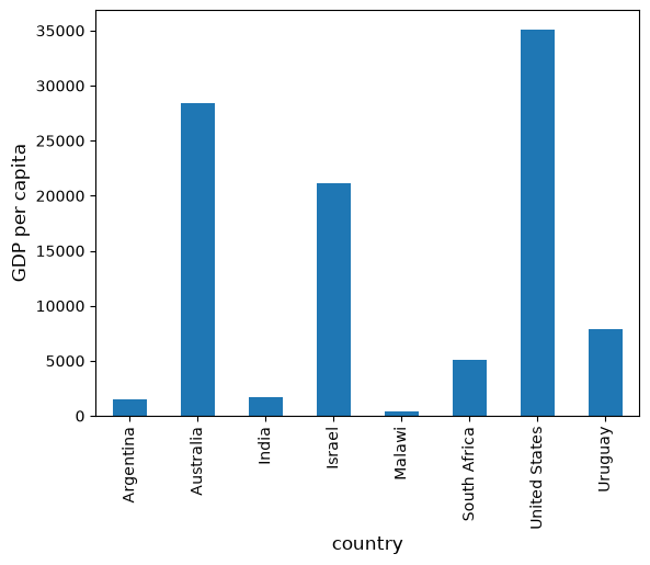
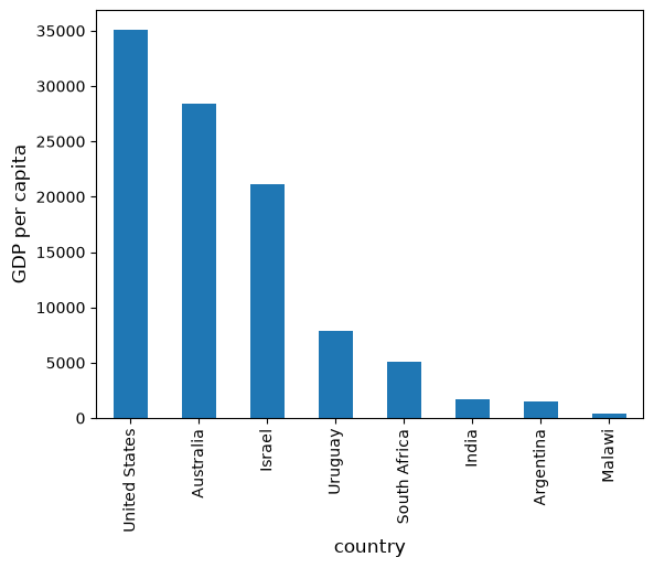
നിലവിൽ data frame countries-ന്റെ alphabetical order-ൽ ആണ് --- നമുക്ക് ഇത് GDP per capita അനുസരിച്ച് മാറ്റാം:
df = df.sort_values(by='GDP percap', ascending=False)
df
| population | total GDP | GDP percap | |
|---|---|---|---|
| country | |||
| United States | 2.821720e+08 | 9.898700e+06 | 35080.381854 |
| Australia | 1.905319e+07 | 5.418047e+05 | 28436.433261 |
| Israel | 6.114570e+06 | 1.292539e+05 | 21138.672749 |
| Uruguay | 3.219793e+06 | 2.525596e+04 | 7843.970620 |
| South Africa | 4.506410e+07 | 2.272424e+05 | 5042.647686 |
| India | 1.006300e+09 | 1.728144e+06 | 1717.324719 |
| Argentina | 1.962465e+08 | 2.950722e+05 | 1503.579625 |
| Malawi | 1.180150e+07 | 5.026222e+03 | 425.896679 |
മുമ്പത്തെപ്പോലെ plot ചെയ്യുമ്പോൾ ഇപ്പോൾ ഇത് ലഭിക്കുന്നു:
ax = df['GDP percap'].plot(kind='bar')
ax.set_xlabel('country', fontsize=12)
ax.set_ylabel('GDP per capita', fontsize=12)
plt.show()
5.4. On-Line Data Sources#
Online databases-നെ programmatically query ചെയ്യുന്നത് Python എളുപ്പമാക്കുന്നു.
Economists-ന് പ്രധാനപ്പെട്ട ഒരു database ആണ് FRED --- St. Louis Fed maintain ചെയ്യുന്ന time series data-യുടെ ഒരു വലിയ collection.
For example, unemployment rate-ൽ നമുക്ക് താൽപ്പര്യമുണ്ടെന്ന് കരുതുക.
(Data-യെ ഒരു csv ആയി download ചെയ്യാൻ, top right-ലുള്ള Download click ചെയ്ത്, CSV (data) എന്ന option select ചെയ്യുക).
ഇതിന് പകരമായി, ഒരു Python program-ന് ഉള്ളിൽ നിന്നും CSV file access ചെയ്യാം.
ഇത് വിവിധ methods ഉപയോഗിച്ച് ചെയ്യാം.
താരതമ്യേന low-level ആയ ഒരു method-ൽ നിന്നും തുടങ്ങി, പിന്നീട് pandas-ഇലേക്ക് നമുക്ക് തിരികെ വരാം.
5.4.1. Accessing Data with requests#
Internet-ൽ നിന്നും data request ചെയ്യാനുള്ള standard Python library ആയ requests ഉപയോഗിക്കുന്നതാണ് ഒരു option.
തുടങ്ങാൻ, നിങ്ങളുടെ computer-ൽ താഴെ പറയുന്ന code try ചെയ്യുക:
r = requests.get('https://fred.stlouisfed.org/graph/fredgraph.csv?bgcolor=%23e1e9f0&chart_type=line&drp=0&fo=open%20sans&graph_bgcolor=%23ffffff&height=450&mode=fred&recession_bars=on&txtcolor=%23444444&ts=12&tts=12&width=1318&nt=0&thu=0&trc=0&show_legend=yes&show_axis_titles=yes&show_tooltip=yes&id=UNRATE&scale=left&cosd=1948-01-01&coed=2024-06-01&line_color=%234572a7&link_values=false&line_style=solid&mark_type=none&mw=3&lw=2&ost=-99999&oet=99999&mma=0&fml=a&fq=Monthly&fam=avg&fgst=lin&fgsnd=2020-02-01&line_index=1&transformation=lin&vintage_date=2024-07-29&revision_date=2024-07-29&nd=1948-01-01')
Error message ഒന്നും ഇല്ലെങ്കിൽ, call വിജയിച്ചു എന്നാണ് അർത്ഥം.
Error ലഭിച്ചാൽ, സാധ്യതയുള്ള രണ്ട് കാരണങ്ങൾ ഇവയാണ്:
നിങ്ങൾ Internet-ഉമായി connect ചെയ്തിട്ടില്ല --- ഇത് അങ്ങനെ അല്ലാതിരിക്കട്ടെ എന്ന് പ്രതീക്ഷിക്കുന്നു.
നിങ്ങളുടെ machine ഒരു proxy server വഴി Internet access ചെയ്യുന്നു, Python-ന് ഇത് അറിയില്ല.
രണ്ടാമത്തെ case-ൽ, നിങ്ങൾക്ക്:
മറ്റൊരു machine-ഇലേക്ക് മാറാം
documentation വായിച്ച് നിങ്ങളുടെ proxy problem പരിഹരിക്കാം
എല്ലാം ശരിയായി പ്രവർത്തിക്കുന്നു എന്ന് കരുതിയാൽ, requests.get(url) എന്ന call return ചെയ്ത data-യിൽ നിന്നും source object build ചെയ്യാൻ ഇപ്പോൾ നിങ്ങൾക്ക് തുടരാം:
url = 'https://fred.stlouisfed.org/graph/fredgraph.csv?bgcolor=%23e1e9f0&chart_type=line&drp=0&fo=open%20sans&graph_bgcolor=%23ffffff&height=450&mode=fred&recession_bars=on&txtcolor=%23444444&ts=12&tts=12&width=1318&nt=0&thu=0&trc=0&show_legend=yes&show_axis_titles=yes&show_tooltip=yes&id=UNRATE&scale=left&cosd=1948-01-01&coed=2024-06-01&line_color=%234572a7&link_values=false&line_style=solid&mark_type=none&mw=3&lw=2&ost=-99999&oet=99999&mma=0&fml=a&fq=Monthly&fam=avg&fgst=lin&fgsnd=2020-02-01&line_index=1&transformation=lin&vintage_date=2024-07-29&revision_date=2024-07-29&nd=1948-01-01'
source = requests.get(url).content.decode().split("\n")
source[0]
'observation_date,UNRATE'
source[1]
'1948-01-01,3.4'
source[2]
'1948-02-01,3.8'
ഈ text parse ചെയ്ത്, ഒരു array ആയി store ചെയ്യാൻ, കുറച്ച് additional code ഇപ്പോൾ നമുക്ക് എഴുതാം.
എന്നാൽ ഇത് ആവശ്യമില്ല --- pandas-ന്റെ read_csv function ഈ task നമുക്കായി handle ചെയ്യും.
Pandas നമ്മുടെ dates column recognize ചെയ്യാൻ, simple date filtering സാധ്യമാക്കാൻ, നമ്മൾ parse_dates=True ഉപയോഗിക്കുന്നു:
data = pd.read_csv(url, index_col=0, parse_dates=True)
data എന്ന ഒരു pandas DataFrame-ഇലേക്ക് data read ചെയ്യപ്പെട്ടിരിക്കുന്നു, ഇപ്പോൾ ഇത് സാധാരണ രീതിയിൽ നമുക്ക് manipulate ചെയ്യാം:
type(data)
pandas.DataFrame
data.head() # A useful method to get a quick look at a data frame
| UNRATE | |
|---|---|
| observation_date | |
| 1948-01-01 | 3.4 |
| 1948-02-01 | 3.8 |
| 1948-03-01 | 4.0 |
| 1948-04-01 | 3.9 |
| 1948-05-01 | 3.5 |
pd.set_option('display.precision', 1)
data.describe()  # Your output might differ slightly
| UNRATE | |
|---|---|
| count | 918.0 |
| mean | 5.7 |
| std | 1.7 |
| min | 2.5 |
| 25% | 4.4 |
| 50% | 5.5 |
| 75% | 6.7 |
| max | 14.8 |
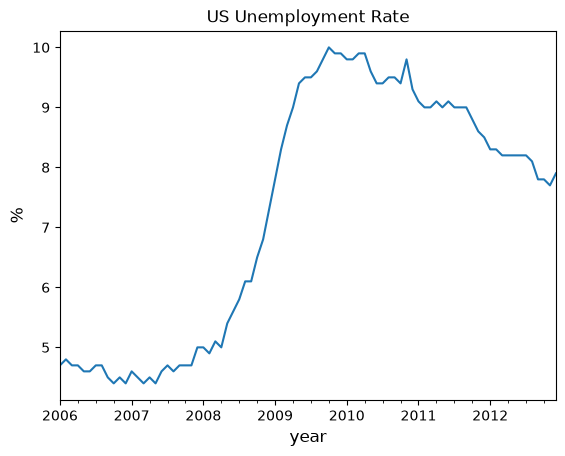
2006 മുതൽ 2012 വരെയുള്ള unemployment rate താഴെ പറയുന്ന വിധത്തിലും നമുക്ക് plot ചെയ്യാം:
ax = data['2006':'2012'].plot(title='US Unemployment Rate', legend=False)
ax.set_xlabel('year', fontsize=12)
ax.set_ylabel('%', fontsize=12)
plt.show()
ശ്രദ്ധിക്കുക, pandas മറ്റ് പല file type alternatives-ഉം നൽകുന്നു.
Data read ചെയ്യാനും, excel, json, parquet-ലേക്കോ database server-ഇലേക്കോ നേരിട്ട് plug ചെയ്യാനും നമുക്ക് ഉപയോഗിക്കാവുന്ന a wide variety top-level methods pandas-ന് ഉണ്ട്.
5.4.2. Using wbgapi and yfinance to Access Data#
World Bank publish ചെയ്യുന്ന പല databases-ൽ നിന്നും data fetch ചെയ്യാൻ wbgapi എന്ന python library ഉപയോഗിക്കാം.
Note
wbgapi package-നെക്കുറിച്ചുള്ള useful ആയ കുറച്ച് information, ഈ tutorial-ന് പുറമേ, ഈ world bank blog post-ലും നിങ്ങൾക്ക് കണ്ടെത്താം
Exercises-ൽ, Yahoo finance-ൽ നിന്നും data fetch ചെയ്യാൻ yfinance-ഉം നമ്മൾ ഉപയോഗിക്കും.
ഇപ്പോൾ, data download ചെയ്ത് plot ചെയ്യുന്നതിന്റെ ഒരു example --- ഇത്തവണ World Bank-ൽ നിന്നും --- നമുക്ക് ചെയ്ത് നോക്കാം.
World Bank, indicators-ന്റെ ഒരു വലിയ range-ലുള്ള data collect ചെയ്ത് organize ചെയ്യുന്നു.
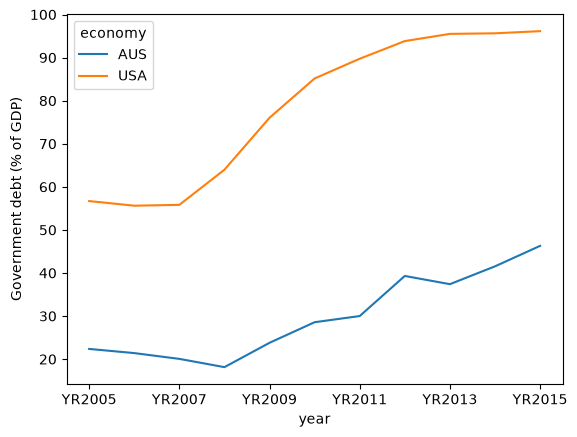
For example, GDP-യുടെ ratio ആയുള്ള government debt-നെക്കുറിച്ചുള്ള കുറച്ച് data ഇവിടെ കാണാം.
അടുത്ത code example, ഈ data നിങ്ങൾക്കായി fetch ചെയ്ത്, US-ന്റെയും Australia-യുടെയും time series plot ചെയ്യുന്നു:
import wbgapi as wb
wb.series.info('GC.DOD.TOTL.GD.ZS')
| id | value |
|---|---|
| GC.DOD.TOTL.GD.ZS | Central government debt, total (% of GDP) |
| 1 elements |
govt_debt = wb.data.DataFrame('GC.DOD.TOTL.GD.ZS', economy=['USA','AUS'], time=range(2005,2016))
govt_debt = govt_debt.T    # move years from columns to rows for plotting
govt_debt.plot(xlabel='year', ylabel='Government debt (% of GDP)');
5.5. Exercises#
Exercise 5.1
With these imports:
import datetime as dt
import yfinance as yf
Write a program to calculate the percentage price change over 2021 for the following shares:
ticker_list = {'INTC': 'Intel',
               'MSFT': 'Microsoft',
               'IBM': 'IBM',
               'BHP': 'BHP',
               'TM': 'Toyota',
               'AAPL': 'Apple',
               'AMZN': 'Amazon',
               'C': 'Citigroup',
               'QCOM': 'Qualcomm',
               'KO': 'Coca-Cola',
               'GOOG': 'Google'}
Here's the first part of the program
def read_data(ticker_list,
          start=dt.datetime(2021, 1, 1),
          end=dt.datetime(2021, 12, 31)):
    """
    This function reads in closing price data from Yahoo
    for each tick in the ticker_list.
    """
    ticker = pd.DataFrame()

    for tick in ticker_list:
        stock = yf.Ticker(tick)
        prices = stock.history(start=start, end=end)

        # Change the index to date-only
        prices.index = pd.to_datetime(prices.index.date)

        closing_prices = prices['Close']
        ticker[tick] = closing_prices

    return ticker

ticker = read_data(ticker_list)
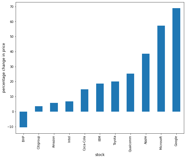
Complete the program to plot the result as a bar graph like this one:
Solution
There are a few ways to approach this problem using Pandas to calculate the percentage change.
First, you can extract the data and perform the calculation such as:
p1 = ticker.iloc[0]    #Get the first set of prices as a Series
p2 = ticker.iloc[-1]   #Get the last set of prices as a Series
price_change = (p2 - p1) / p1 * 100
price_change
INTC     6.9
MSFT    57.2
IBM     18.7
BHP     -2.2
TM      23.4
AAPL    38.6
AMZN     5.8
C        3.6
QCOM    25.3
KO      14.9
GOOG    69.0
dtype: float64
Alternatively you can use an inbuilt method pct_change and configure it to
perform the correct calculation using periods argument.
change = ticker.pct_change(periods=len(ticker)-1, axis='rows')*100
price_change = change.iloc[-1]
price_change
INTC     6.9
MSFT    57.2
IBM     18.7
BHP     -2.2
TM      23.4
AAPL    38.6
AMZN     5.8
C        3.6
QCOM    25.3
KO      14.9
GOOG    69.0
Name: 2021-12-30 00:00:00, dtype: float64
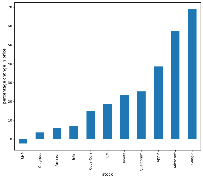
Then to plot the chart
price_change.sort_values(inplace=True)
price_change.rename(index=ticker_list, inplace=True)
fig, ax = plt.subplots(figsize=(10,8))
ax.set_xlabel('stock', fontsize=12)
ax.set_ylabel('percentage change in price', fontsize=12)
price_change.plot(kind='bar', ax=ax)
plt.show()
Exercise 5.2
Using the method read_data introduced in Exercise 5.1, write a program to obtain year-on-year percentage change for the following indices:
indices_list = {'^GSPC': 'S&P 500',
               '^IXIC': 'NASDAQ',
               '^DJI': 'Dow Jones',
               '^N225': 'Nikkei'}
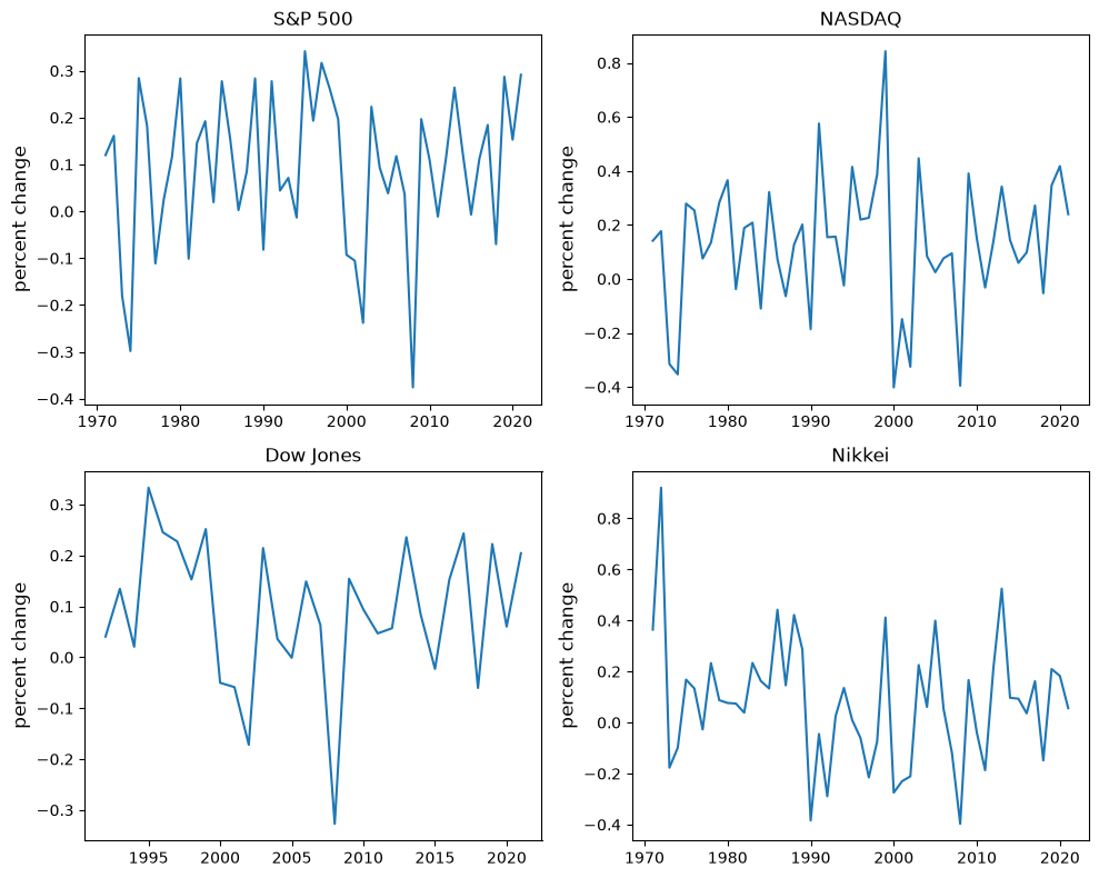
Complete the program to show summary statistics and plot the result as a time series graph like this one:
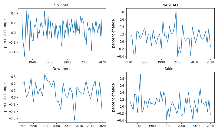
Solution
Following the work you did in Exercise 5.1, you can query the data using read_data by updating the start and end dates accordingly.
indices_data = read_data(
        indices_list,
        start=dt.datetime(1971, 1, 1),  #Common Start Date
        end=dt.datetime(2021, 12, 31)
)
Then, extract the first and last set of prices per year as DataFrames and calculate the yearly returns such as:
yearly_returns = pd.DataFrame()

for index, name in indices_list.items():
    p1 = indices_data.groupby(indices_data.index.year)[index].first()  # Get the first set of returns as a DataFrame
    p2 = indices_data.groupby(indices_data.index.year)[index].last()   # Get the last set of returns as a DataFrame
    returns = (p2 - p1) / p1
    yearly_returns[name] = returns

yearly_returns
| S&P 500 | NASDAQ | Dow Jones | Nikkei | |
|---|---|---|---|---|
| 1971 | 1.2e-01 | 1.4e-01 | NaN | 3.6e-01 |
| 1972 | 1.6e-01 | 1.8e-01 | NaN | 9.2e-01 |
| 1973 | -1.8e-01 | -3.2e-01 | NaN | -1.8e-01 |
| 1974 | -3.0e-01 | -3.5e-01 | NaN | -9.9e-02 |
| 1975 | 2.8e-01 | 2.8e-01 | NaN | 1.7e-01 |
| 1976 | 1.8e-01 | 2.5e-01 | NaN | 1.3e-01 |
| 1977 | -1.1e-01 | 7.5e-02 | NaN | -2.7e-02 |
| 1978 | 2.4e-02 | 1.3e-01 | NaN | 2.3e-01 |
| 1979 | 1.2e-01 | 2.8e-01 | NaN | 8.7e-02 |
| 1980 | 2.8e-01 | 3.7e-01 | NaN | 7.7e-02 |
| 1981 | -1.0e-01 | -3.8e-02 | NaN | 7.4e-02 |
| 1982 | 1.5e-01 | 1.9e-01 | NaN | 3.9e-02 |
| 1983 | 1.9e-01 | 2.1e-01 | NaN | 2.3e-01 |
| 1984 | 2.0e-02 | -1.1e-01 | NaN | 1.6e-01 |
| 1985 | 2.8e-01 | 3.2e-01 | NaN | 1.3e-01 |
| 1986 | 1.6e-01 | 7.3e-02 | NaN | 4.4e-01 |
| 1987 | 2.6e-03 | -6.4e-02 | NaN | 1.5e-01 |
| 1988 | 8.5e-02 | 1.3e-01 | NaN | 4.2e-01 |
| 1989 | 2.8e-01 | 2.0e-01 | NaN | 2.9e-01 |
| 1990 | -8.2e-02 | -1.9e-01 | NaN | -3.8e-01 |
| 1991 | 2.8e-01 | 5.8e-01 | NaN | -4.5e-02 |
| 1992 | 4.4e-02 | 1.5e-01 | 4.1e-02 | -2.9e-01 |
| 1993 | 7.1e-02 | 1.6e-01 | 1.3e-01 | 2.5e-02 |
| 1994 | -1.3e-02 | -2.4e-02 | 2.1e-02 | 1.4e-01 |
| 1995 | 3.4e-01 | 4.1e-01 | 3.3e-01 | 9.4e-03 |
| 1996 | 1.9e-01 | 2.2e-01 | 2.5e-01 | -6.1e-02 |
| 1997 | 3.2e-01 | 2.3e-01 | 2.3e-01 | -2.2e-01 |
| 1998 | 2.6e-01 | 3.9e-01 | 1.5e-01 | -7.5e-02 |
| 1999 | 2.0e-01 | 8.4e-01 | 2.5e-01 | 4.1e-01 |
| 2000 | -9.3e-02 | -4.0e-01 | -5.0e-02 | -2.7e-01 |
| 2001 | -1.1e-01 | -1.5e-01 | -5.9e-02 | -2.3e-01 |
| 2002 | -2.4e-01 | -3.3e-01 | -1.7e-01 | -2.1e-01 |
| 2003 | 2.2e-01 | 4.5e-01 | 2.1e-01 | 2.3e-01 |
| 2004 | 9.3e-02 | 8.4e-02 | 3.6e-02 | 6.1e-02 |
| 2005 | 3.8e-02 | 2.5e-02 | -1.1e-03 | 4.0e-01 |
| 2006 | 1.2e-01 | 7.6e-02 | 1.5e-01 | 5.3e-02 |
| 2007 | 3.7e-02 | 9.5e-02 | 6.3e-02 | -1.2e-01 |
| 2008 | -3.8e-01 | -4.0e-01 | -3.3e-01 | -4.0e-01 |
| 2009 | 2.0e-01 | 3.9e-01 | 1.5e-01 | 1.7e-01 |
| 2010 | 1.1e-01 | 1.5e-01 | 9.4e-02 | -4.0e-02 |
| 2011 | -1.1e-02 | -3.2e-02 | 4.7e-02 | -1.9e-01 |
| 2012 | 1.2e-01 | 1.4e-01 | 5.7e-02 | 2.1e-01 |
| 2013 | 2.6e-01 | 3.4e-01 | 2.4e-01 | 5.2e-01 |
| 2014 | 1.2e-01 | 1.4e-01 | 8.4e-02 | 9.7e-02 |
| 2015 | -6.9e-03 | 5.9e-02 | -2.3e-02 | 9.3e-02 |
| 2016 | 1.1e-01 | 9.8e-02 | 1.5e-01 | 3.6e-02 |
| 2017 | 1.8e-01 | 2.7e-01 | 2.4e-01 | 1.6e-01 |
| 2018 | -7.0e-02 | -5.3e-02 | -6.0e-02 | -1.5e-01 |
| 2019 | 2.9e-01 | 3.5e-01 | 2.2e-01 | 2.1e-01 |
| 2020 | 1.5e-01 | 4.2e-01 | 6.0e-02 | 1.8e-01 |
| 2021 | 2.9e-01 | 2.4e-01 | 2.0e-01 | 5.6e-02 |
Next, you can obtain summary statistics by using the method describe.
yearly_returns.describe()
| S&P 500 | NASDAQ | Dow Jones | Nikkei | |
|---|---|---|---|---|
| count | 5.1e+01 | 5.1e+01 | 3.0e+01 | 5.1e+01 |
| mean | 9.2e-02 | 1.3e-01 | 9.1e-02 | 7.9e-02 |
| std | 1.6e-01 | 2.5e-01 | 1.4e-01 | 2.4e-01 |
| min | -3.8e-01 | -4.0e-01 | -3.3e-01 | -4.0e-01 |
| 25% | -2.2e-03 | 1.6e-04 | 2.5e-02 | -6.8e-02 |
| 50% | 1.2e-01 | 1.4e-01 | 8.9e-02 | 7.7e-02 |
| 75% | 2.0e-01 | 2.8e-01 | 2.1e-01 | 2.0e-01 |
| max | 3.4e-01 | 8.4e-01 | 3.3e-01 | 9.2e-01 |
Then, to plot the chart
fig, axes = plt.subplots(2, 2, figsize=(10, 8))

for iter_, ax in enumerate(axes.flatten()):            # Flatten 2-D array to 1-D array
    index_name = yearly_returns.columns[iter_]         # Get index name per iteration
    ax.plot(yearly_returns[index_name])                # Plot pct change of yearly returns per index
    ax.set_ylabel("percent change", fontsize = 12)
    ax.set_title(index_name)

plt.tight_layout()