3. Matplotlib#

3.1. Overview#

ഈ lectures-ൽ Matplotlib ഉപയോഗിച്ച് നമ്മൾ ഇതിനകം ധാരാളം figures generate ചെയ്തിട്ടുണ്ട്.

Matplotlib എന്നത് scientific computing-നു വേണ്ടി design ചെയ്ത ഒരു മികച്ച graphics library ആണ്, അതിൽ ഇവയുണ്ട്:

  • high-quality 2D, 3D plots

  • സാധാരണ formats-ലെല്ലാമുള്ള output (PDF, PNG മുതലായവ)

  • LaTeX integration

  • presentation-ന്റെ എല്ലാ വശങ്ങളിലും fine-grained control

  • animation മുതലായവ

3.1.1. Matplotlib's Split Personality#

Matplotlib വ്യത്യസ്തമായത് അത് plotting-ന് രണ്ട് വ്യത്യസ്ത interfaces provide ചെയ്യുന്നു എന്നതിലാണ്.

ഒന്ന്, MATLAB refugees-ന് ഒരു ready home കണ്ടെത്താൻ സഹായിക്കാൻ വേണ്ടി എഴുതിയ simple ആയ MATLAB-style API (Application Programming Interface) ആണ്.

മറ്റൊന്ന് കൂടുതൽ "Pythonic" ആയ object-oriented API ആണ്.

താഴെ വിവരിക്കുന്ന കാരണങ്ങളാൽ, രണ്ടാമത്തെ API ഉപയോഗിക്കാൻ ഞങ്ങൾ recommend ചെയ്യുന്നു.

പക്ഷേ ആദ്യം, ഈ വ്യത്യാസം എന്താണെന്ന് നോക്കാം.

3.2. The APIs#

3.2.1. The MATLAB-style API#

Introductory treatments-ൽ കാണാൻ സാധ്യതയുള്ള ഒരു easy ആയ example താഴെ കാണാം:

import matplotlib.pyplot as plt
import numpy as np

x = np.linspace(0, 10, 200)
y = np.sin(x)

plt.plot(x, y, 'b-', linewidth=2)
plt.show()
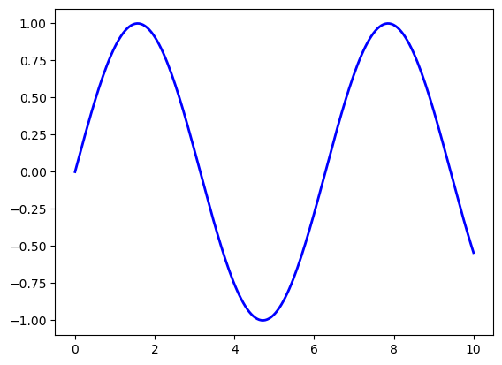
_images/abeb4cb1edbad1dc9730e37d6bcdeed8be3806eeccdfde6decf42c64cc1d5f22.png

ഇത് simple-ഉം convenient-ഉം ആണ്, പക്ഷേ ഇതിന് ചില പരിമിതികളുണ്ട്, മാത്രമല്ല ഇത് un-Pythonic ആണ്.

For example, function calls-ൽ, programmer-നെ അറിയിക്കാതെ തന്നെ ധാരാളം objects create ചെയ്യപ്പെടുകയും pass ചെയ്യപ്പെടുകയും ചെയ്യുന്നു.

Python programmers സാധാരണയായി കൂടുതൽ explicit ആയ ഒരു programming style ആണ് preferചെയ്യുന്നത് (ഒരു code block-ൽ import this run ചെയ്ത് രണ്ടാമത്തെ line നോക്കുക).

ഇത് നമ്മെ ഒരു alternative ആയ, object-oriented Matplotlib API-യിലേക്ക് നയിക്കുന്നു.

3.2.2. The Object-Oriented API#

Object-oriented API ഉപയോഗിച്ച്, മുമ്പത്തെ figure-നു അനുയോജ്യമായ code താഴെ കാണാം:

fig, ax = plt.subplots()
ax.plot(x, y, 'b-', linewidth=2)
plt.show()
_images/abeb4cb1edbad1dc9730e37d6bcdeed8be3806eeccdfde6decf42c64cc1d5f22.png

ഇവിടെ fig, ax = plt.subplots() എന്ന call ഒരു pair return ചെയ്യുന്നു, അതിൽ:

  • fig ഒരു Figure instance ആണ് --- ഒരു blank canvas പോലെ.

  • ax ഒരു AxesSubplot instance ആണ് --- plotting ചെയ്യാനുള്ള ഒരു frame ആയി കരുതുക.

plot() function യഥാർത്ഥത്തിൽ ax-ന്റെ ഒരു method ആണ്.

കുറച്ചുകൂടി typing വേണ്ടിവരുമെങ്കിലും, objects-ന്റെ കൂടുതൽ explicit ആയ ഉപയോഗം നമുക്ക് കൂടുതൽ നല്ല control നൽകുന്നു.

നമ്മൾ മുന്നോട്ട് പോകുമ്പോൾ ഇത് കൂടുതൽ വ്യക്തമാകും.

3.2.3. Tweaks#

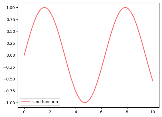
ഇവിടെ നമ്മൾ line-ന്റെ നിറം red ആക്കി മാറ്റുകയും ഒരു legend ചേർക്കുകയും ചെയ്തിരിക്കുന്നു:

fig, ax = plt.subplots()
ax.plot(x, y, 'r-', linewidth=2, label='sine function', alpha=0.6)
ax.legend()
plt.show()
_images/7e3a98583ea39e43c755f2c54ff3d82f74475cbdbbe7cdb35eea1f84befbecaa.png

Line-നെ അല്പം transparent ആക്കാൻ നമ്മൾ alpha ഉപയോഗിച്ചിട്ടുണ്ട് --- ഇത് അതിനെ smooth ആയി കാണിക്കുന്നു.

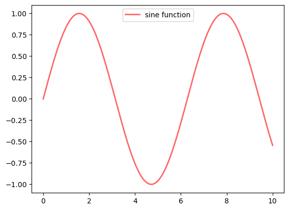
ax.legend()-നെ ax.legend(loc='upper center') ഉപയോഗിച്ച് മാറ്റി legend-ന്റെ സ്ഥാനം മാറ്റാൻ സാധിക്കും.

fig, ax = plt.subplots()
ax.plot(x, y, 'r-', linewidth=2, label='sine function', alpha=0.6)
ax.legend(loc='upper center')
plt.show()
_images/b0ca63d819bd043d4227e0400cd82dbe02214dd0d99b3ffdcfb80469dcde5529.png

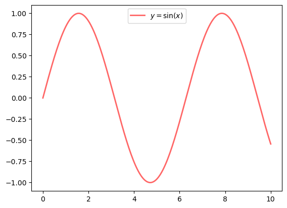
എല്ലാം ശരിയായി configure ചെയ്തിട്ടുണ്ടെങ്കിൽ, LaTeX ചേർക്കുന്നത് വളരെ എളുപ്പം ആണ്:

fig, ax = plt.subplots()
ax.plot(x, y, 'r-', linewidth=2, label=r'$y=\sin(x)$', alpha=0.6)
ax.legend(loc='upper center')
plt.show()
_images/e15823f6ed52a8c26dc57d2fab36459da1c66ba7ccc727be2420cd6f37565bf5.png

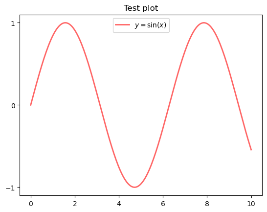
Ticks control ചെയ്യുന്നതും titles ചേർക്കുന്നതും മറ്റും also എളുപ്പം ആണ്:

fig, ax = plt.subplots()
ax.plot(x, y, 'r-', linewidth=2, label=r'$y=\sin(x)$', alpha=0.6)
ax.legend(loc='upper center')
ax.set_yticks([-1, 0, 1])
ax.set_title('Test plot')
plt.show()
_images/f9527268d7e35e69d0fc3c5dfefeca7db3460bbf10a7812e7e9d1b77c3da22c0.png

3.3. More Features#

Matplotlib-ന് വളരെ വലിയ ഒരു functions-ന്റെ ഒപ്പം features-ന്റെ collection ഉണ്ട്, ആവശ്യമായി വരുമ്പോൾ കാലക്രമേണ നിങ്ങൾ അവ discover ചെയ്യും.

അതിൽ ചിലത് മാത്രം ഇവിടെ പറയാം.

3.3.1. Multiple Plots on One Axis#

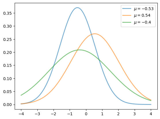
ഒരേ axes-ൽ multiple plots generate ചെയ്യുന്നത് വളരെ എളുപ്പം ആണ്.

Random ആയി മൂന്ന് normal densities generate ചെയ്ത് അവയുടെ mean-ഉള്ള ഒരു label ചേർക്കുന്ന example താഴെ കാണാം:

from scipy.stats import norm
from random import uniform

fig, ax = plt.subplots()
x = np.linspace(-4, 4, 150)
for i in range(3):
    m, s = uniform(-1, 1), uniform(1, 2)
    y = norm.pdf(x, loc=m, scale=s)
    current_label = rf'$\mu = {m:.2}$'
    ax.plot(x, y, linewidth=2, alpha=0.6, label=current_label)
ax.legend()
plt.show()
_images/36b38a1fb2a09565d95e42bab4d9f285376a619efd26cf6e36596eee184077f2.png

3.3.2. Multiple Subplots#

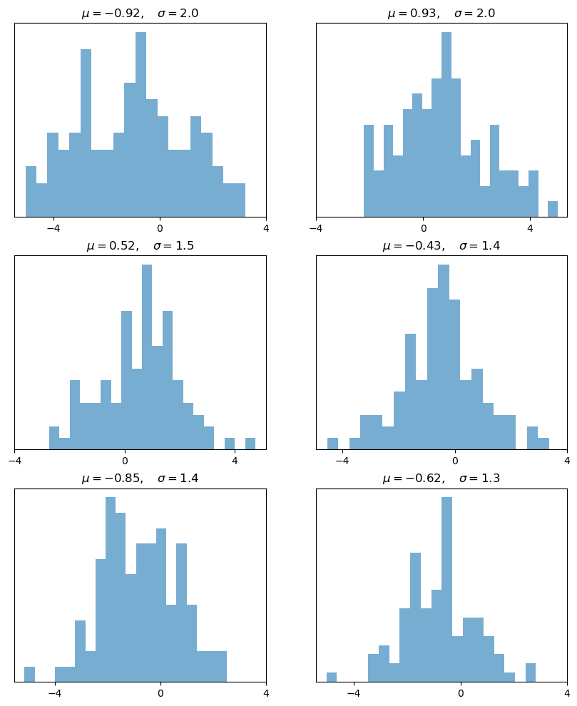
ചിലപ്പോൾ നമുക്ക് ഒരു figure-ൽ multiple subplots വേണ്ടിവരും.

6 histograms generate ചെയ്യുന്ന ഒരു example താഴെ കാണാം:

num_rows, num_cols = 3, 2
fig, axes = plt.subplots(num_rows, num_cols, figsize=(10, 12))
for i in range(num_rows):
    for j in range(num_cols):
        m, s = uniform(-1, 1), uniform(1, 2)
        x = norm.rvs(loc=m, scale=s, size=100)
        axes[i, j].hist(x, alpha=0.6, bins=20)
        t = rf'$\mu = {m:.2}, \quad \sigma = {s:.2}$'
        axes[i, j].set(title=t, xticks=[-4, 0, 4], yticks=[])
plt.show()
_images/606d88b0107b0b229a5809dc68013b80aba651bec6635f362674f993e25bd6fb.png

3.3.3. 3D Plots#

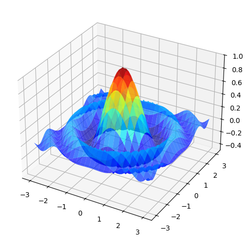
Matplotlib 3D plots-ന്റെ കാര്യത്തിലും നല്ല ജോലി ചെയ്യുന്നു --- ഒരു example താഴെ കാണാം:

from mpl_toolkits.mplot3d.axes3d import Axes3D
from matplotlib import cm


def f(x, y):
    return np.cos(x**2 + y**2) / (1 + x**2 + y**2)

xgrid = np.linspace(-3, 3, 50)
ygrid = xgrid
x, y = np.meshgrid(xgrid, ygrid)

fig = plt.figure(figsize=(10, 6))
ax = fig.add_subplot(111, projection='3d')
ax.plot_surface(x,
                y,
                f(x, y),
                rstride=2, cstride=2,
                cmap=cm.jet,
                alpha=0.7,
                linewidth=0.25)
ax.set_zlim(-0.5, 1.0)
plt.show()
_images/8e79260b1d892170b9c2017fa016e9ffcbf12e632c5f94ca04ae4aa3e6c6e679.png

3.3.4. A Customizing Function#

ഒരു set of customizations നിങ്ങൾ സ്ഥിരമായി ഉപയോഗിക്കുന്നത് കണ്ടെത്തിയേക്കാം.

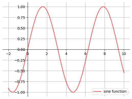
നമ്മുടെ axes origin-ലൂടെ പോകണം എന്നും, ഒരു grid ഉണ്ടാകണം എന്നും നമ്മൾ സാധാരണയായി preferചെയ്യുന്നു എന്ന് കരുതുക.

ഈ മാറ്റങ്ങൾ implement ചെയ്യുന്ന ഒരു custom subplots function build ചെയ്യാൻ object-oriented API എങ്ങനെ ഉപയോഗിക്കാം എന്നതിന്റെ ഒരു നല്ല example Matthew Doty-യിൽ നിന്നും താഴെ കാണാം.

Code ശ്രദ്ധയോടെ വായിച്ച്, എന്താണ് നടക്കുന്നത് എന്ന് follow ചെയ്യാൻ കഴിയുമോ എന്ന് നോക്കുക:

def subplots():
    "Custom subplots with axes through the origin"
    fig, ax = plt.subplots()

    # Set the axes through the origin
    for spine in ['left', 'bottom']:
        ax.spines[spine].set_position('zero')
    for spine in ['right', 'top']:
        ax.spines[spine].set_color('none')

    ax.grid()
    return fig, ax


fig, ax = subplots()  # Call the local version, not plt.subplots()
x = np.linspace(-2, 10, 200)
y = np.sin(x)
ax.plot(x, y, 'r-', linewidth=2, label='sine function', alpha=0.6)
ax.legend(loc='lower right')
plt.show()
_images/7a844547d1a123077a37802077a36361f9f38008f11f1a867d2fce09bd3323ad.png

Custom subplots function:

  1. fig, ax pair generate ചെയ്യാൻ internal ആയി standard plt.subplots function-നെ call ചെയ്യുന്നു,

  2. ax-ൽ ആവശ്യമായ customizations വരുത്തുന്നു, ഒപ്പം

  3. fig, ax pair-നെ calling code-ലേക്ക് pass ചെയ്ത് തിരികെ നൽകുന്നു.

3.3.5. Style Sheets#

Matplotlib-ലെ മറ്റൊരു വളരെ useful ആയ feature ആണ് style sheets.

Uniform ആയ styles ഉള്ള plots create ചെയ്യാൻ നമുക്ക് style sheets ഉപയോഗിക്കാം.

plt.style.available എന്ന attribute print ചെയ്ത് available styles-ന്റെ ഒരു list നമുക്ക് കണ്ടെത്താം:

print(plt.style.available)
['Solarize_Light2', '_classic_test_patch', '_mpl-gallery', '_mpl-gallery-nogrid', 'bmh', 'classic', 'dark_background', 'fast', 'fivethirtyeight', 'ggplot', 'grayscale', 'petroff10', 'seaborn-v0_8', 'seaborn-v0_8-bright', 'seaborn-v0_8-colorblind', 'seaborn-v0_8-dark', 'seaborn-v0_8-dark-palette', 'seaborn-v0_8-darkgrid', 'seaborn-v0_8-deep', 'seaborn-v0_8-muted', 'seaborn-v0_8-notebook', 'seaborn-v0_8-paper', 'seaborn-v0_8-pastel', 'seaborn-v0_8-poster', 'seaborn-v0_8-talk', 'seaborn-v0_8-ticks', 'seaborn-v0_8-white', 'seaborn-v0_8-whitegrid', 'tableau-colorblind10']

ഇനി style sheet set ചെയ്യാൻ നമുക്ക് plt.style.use() method ഉപയോഗിക്കാം.

ഒരു style sheet-ന്റെ പേര് എടുത്ത് ആ style ഉപയോഗിച്ച് വ്യത്യസ്ത plots വരയ്ക്കുന്ന ഒരു function നമുക്ക് എഴുതാം:

def draw_graphs(style='default'):

    # Setting a style sheet
    plt.style.use(style)

    fig, axes = plt.subplots(nrows=1, ncols=4, figsize=(10, 3))
    x = np.linspace(-13, 13, 150)

    # Set seed values to replicate results of random draws
    np.random.seed(9)

    for i in range(3):

        # Draw mean and standard deviation from uniform distributions
        m, s = np.random.uniform(-8, 8), np.random.uniform(2, 2.5)

        # Generate a normal density plot
        y = norm.pdf(x, loc=m, scale=s)
        axes[0].plot(x, y, linewidth=3, alpha=0.7)

        # Create a scatter plot with random X and Y values 
        # from normal distributions
        rnormX = norm.rvs(loc=m, scale=s, size=150)
        rnormY = norm.rvs(loc=m, scale=s, size=150)
        axes[1].plot(rnormX, rnormY, ls='none', marker='o', alpha=0.7)

        # Create a histogram with random X values
        axes[2].hist(rnormX, alpha=0.7)

        # and a line graph with random Y values
        axes[3].plot(x, rnormY, linewidth=2, alpha=0.7)

    style_name = style.split('-')[0]
    plt.suptitle(f'Style: {style_name}', fontsize=13)
    plt.show()

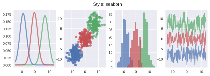
ഈ styles-ൽ ചിലത് എങ്ങനെ കാണപ്പെടുന്നു എന്ന് നോക്കാം.

ആദ്യം, seaborn എന്ന style sheet ഉപയോഗിച്ച് graphs വരയ്ക്കാം:

draw_graphs(style='seaborn-v0_8')
_images/26ee097a74e5fd4d69fbc06b454b87c2704222bf9976aef254e72040a7b5ffa9.png

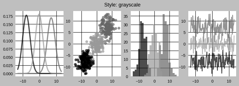
Plots-ലെ colors ഒഴിവാക്കാൻ നമുക്ക് grayscale ഉപയോഗിക്കാം:

draw_graphs(style='grayscale')
_images/9c1a5d4b452e10ac6b5d427ef1b066ebc211c0dab11f13021915adf44a5e6d06.png

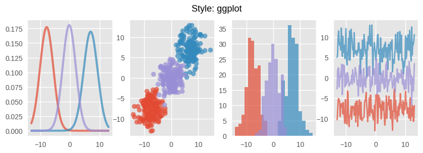
ggplot എങ്ങനെ കാണപ്പെടുന്നു എന്ന് താഴെ കാണാം:

draw_graphs(style='ggplot')
_images/45645d591910f4d2d63d4d3c9d24b9b219e7b644286701faedc8388bfa7eeb16.png

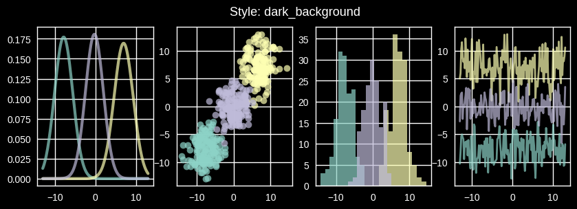
നമുക്ക് dark_background എന്ന style-ഉം ഉപയോഗിക്കാം:

draw_graphs(style='dark_background')
_images/56f017ba6c9afc48a59575a9c70cea8bf374faade5f51e2338b404c3a57d5a78.png

List-ലെ മറ്റ് styles experiment ചെയ്യാൻ നിങ്ങൾക്ക് ഈ function ഉപയോഗിക്കാം.

നിങ്ങൾക്ക് താൽപ്പര്യമുണ്ടെങ്കിൽ, നിങ്ങളുടെ own style sheets തന്നെ create ചെയ്യാം.

നിങ്ങളുടെ style sheets-ന്റെ parameters plt.rcParams എന്ന dictionary-like variable-ൽ store ചെയ്യപ്പെടുന്നു:

print(plt.rcParams.keys())

Hide code cell output

KeysView(RcParams({'_internal.classic_mode': False,
          'agg.path.chunksize': 0,
          'animation.bitrate': -1,
          'animation.codec': 'h264',
          'animation.convert_args': ['-layers', 'OptimizePlus'],
          'animation.convert_path': 'convert',
          'animation.embed_limit': 20.0,
          'animation.ffmpeg_args': [],
          'animation.ffmpeg_path': 'ffmpeg',
          'animation.frame_format': 'png',
          'animation.html': 'none',
          'animation.writer': 'ffmpeg',
          'axes.autolimit_mode': 'data',
          'axes.axisbelow': True,
          'axes.edgecolor': 'white',
          'axes.facecolor': 'black',
          'axes.formatter.limits': [-5, 6],
          'axes.formatter.min_exponent': 0,
          'axes.formatter.offset_threshold': 4,
          'axes.formatter.use_locale': False,
          'axes.formatter.use_mathtext': False,
          'axes.formatter.useoffset': True,
          'axes.grid': True,
          'axes.grid.axis': 'both',
          'axes.grid.which': 'major',
          'axes.labelcolor': 'white',
          'axes.labelpad': 4.0,
          'axes.labelsize': 'large',
          'axes.labelweight': 'normal',
          'axes.linewidth': 1.0,
          'axes.prop_cycle': cycler('color', ['#8dd3c7', '#feffb3', '#bfbbd9', '#fa8174', '#81b1d2', '#fdb462', '#b3de69', '#bc82bd', '#ccebc4', '#ffed6f']),
          'axes.spines.bottom': True,
          'axes.spines.left': True,
          'axes.spines.right': True,
          'axes.spines.top': True,
          'axes.titlecolor': 'auto',
          'axes.titlelocation': 'center',
          'axes.titlepad': 6.0,
          'axes.titlesize': 'x-large',
          'axes.titleweight': 'normal',
          'axes.titley': None,
          'axes.unicode_minus': True,
          'axes.xmargin': 0.05,
          'axes.ymargin': 0.05,
          'axes.zmargin': 0.05,
          'axes3d.automargin': False,
          'axes3d.grid': True,
          'axes3d.mouserotationstyle': 'arcball',
          'axes3d.trackballborder': 0.2,
          'axes3d.trackballsize': 0.667,
          'axes3d.xaxis.panecolor': (0.95, 0.95, 0.95, 0.5),
          'axes3d.yaxis.panecolor': (0.9, 0.9, 0.9, 0.5),
          'axes3d.zaxis.panecolor': (0.925, 0.925, 0.925, 0.5),
          'backend': 'module://matplotlib_inline.backend_inline',
          'backend_fallback': True,
          'boxplot.bootstrap': None,
          'boxplot.boxprops.color': 'white',
          'boxplot.boxprops.linestyle': '-',
          'boxplot.boxprops.linewidth': 1.0,
          'boxplot.capprops.color': 'white',
          'boxplot.capprops.linestyle': '-',
          'boxplot.capprops.linewidth': 1.0,
          'boxplot.flierprops.color': 'white',
          'boxplot.flierprops.linestyle': 'none',
          'boxplot.flierprops.linewidth': 1.0,
          'boxplot.flierprops.marker': 'o',
          'boxplot.flierprops.markeredgecolor': 'white',
          'boxplot.flierprops.markeredgewidth': 1.0,
          'boxplot.flierprops.markerfacecolor': 'none',
          'boxplot.flierprops.markersize': 6.0,
          'boxplot.meanline': False,
          'boxplot.meanprops.color': 'C2',
          'boxplot.meanprops.linestyle': '--',
          'boxplot.meanprops.linewidth': 1.0,
          'boxplot.meanprops.marker': '^',
          'boxplot.meanprops.markeredgecolor': 'C2',
          'boxplot.meanprops.markerfacecolor': 'C2',
          'boxplot.meanprops.markersize': 6.0,
          'boxplot.medianprops.color': 'C1',
          'boxplot.medianprops.linestyle': '-',
          'boxplot.medianprops.linewidth': 1.0,
          'boxplot.notch': False,
          'boxplot.patchartist': False,
          'boxplot.showbox': True,
          'boxplot.showcaps': True,
          'boxplot.showfliers': True,
          'boxplot.showmeans': False,
          'boxplot.vertical': True,
          'boxplot.whiskerprops.color': 'white',
          'boxplot.whiskerprops.linestyle': '-',
          'boxplot.whiskerprops.linewidth': 1.0,
          'boxplot.whiskers': 1.5,
          'contour.algorithm': 'mpl2014',
          'contour.corner_mask': True,
          'contour.linewidth': None,
          'contour.negative_linestyle': 'dashed',
          'date.autoformatter.day': '%Y-%m-%d',
          'date.autoformatter.hour': '%m-%d %H',
          'date.autoformatter.microsecond': '%M:%S.%f',
          'date.autoformatter.minute': '%d %H:%M',
          'date.autoformatter.month': '%Y-%m',
          'date.autoformatter.second': '%H:%M:%S',
          'date.autoformatter.year': '%Y',
          'date.converter': 'auto',
          'date.epoch': '1970-01-01T00:00:00',
          'date.interval_multiples': True,
          'docstring.hardcopy': False,
          'errorbar.capsize': 0.0,
          'figure.autolayout': False,
          'figure.constrained_layout.h_pad': 0.04167,
          'figure.constrained_layout.hspace': 0.02,
          'figure.constrained_layout.use': False,
          'figure.constrained_layout.w_pad': 0.04167,
          'figure.constrained_layout.wspace': 0.02,
          'figure.dpi': 100.0,
          'figure.edgecolor': 'black',
          'figure.facecolor': 'black',
          'figure.figsize': [8.0, 5.5],
          'figure.frameon': True,
          'figure.hooks': [],
          'figure.labelsize': 'large',
          'figure.labelweight': 'normal',
          'figure.max_open_warning': 20,
          'figure.raise_window': True,
          'figure.subplot.bottom': 0.11,
          'figure.subplot.hspace': 0.2,
          'figure.subplot.left': 0.125,
          'figure.subplot.right': 0.9,
          'figure.subplot.top': 0.88,
          'figure.subplot.wspace': 0.2,
          'figure.titlesize': 'large',
          'figure.titleweight': 'normal',
          'font.cursive': ['Apple Chancery',
                           'Textile',
                           'Zapf Chancery',
                           'Sand',
                           'Script MT',
                           'Felipa',
                           'Comic Neue',
                           'Comic Sans MS',
                           'cursive'],
          'font.family': ['sans-serif'],
          'font.fantasy': ['Chicago',
                           'Charcoal',
                           'Impact',
                           'Western',
                           'xkcd script',
                           'fantasy'],
          'font.monospace': ['DejaVu Sans Mono',
                             'Bitstream Vera Sans Mono',
                             'Computer Modern Typewriter',
                             'Andale Mono',
                             'Nimbus Mono L',
                             'Courier New',
                             'Courier',
                             'Fixed',
                             'Terminal',
                             'monospace'],
          'font.sans-serif': ['Arial',
                              'Liberation Sans',
                              'DejaVu Sans',
                              'Bitstream Vera Sans',
                              'sans-serif'],
          'font.serif': ['DejaVu Serif',
                         'Bitstream Vera Serif',
                         'Computer Modern Roman',
                         'New Century Schoolbook',
                         'Century Schoolbook L',
                         'Utopia',
                         'ITC Bookman',
                         'Bookman',
                         'Nimbus Roman No9 L',
                         'Times New Roman',
                         'Times',
                         'Palatino',
                         'Charter',
                         'serif'],
          'font.size': 10.0,
          'font.stretch': 'normal',
          'font.style': 'normal',
          'font.variant': 'normal',
          'font.weight': 'normal',
          'grid.alpha': 1.0,
          'grid.color': 'white',
          'grid.linestyle': '-',
          'grid.linewidth': 1.0,
          'hatch.color': 'black',
          'hatch.linewidth': 1.0,
          'hist.bins': 10,
          'image.aspect': 'equal',
          'image.cmap': 'gray',
          'image.composite_image': True,
          'image.interpolation': 'auto',
          'image.interpolation_stage': 'auto',
          'image.lut': 256,
          'image.origin': 'upper',
          'image.resample': True,
          'interactive': True,
          'keymap.back': ['left', 'c', 'backspace', 'MouseButton.BACK'],
          'keymap.copy': ['ctrl+c', 'cmd+c'],
          'keymap.forward': ['right', 'v', 'MouseButton.FORWARD'],
          'keymap.fullscreen': ['f', 'ctrl+f'],
          'keymap.grid': ['g'],
          'keymap.grid_minor': ['G'],
          'keymap.help': ['f1'],
          'keymap.home': ['h', 'r', 'home'],
          'keymap.pan': ['p'],
          'keymap.quit': ['ctrl+w', 'cmd+w', 'q'],
          'keymap.quit_all': [],
          'keymap.save': ['s', 'ctrl+s'],
          'keymap.xscale': ['k', 'L'],
          'keymap.yscale': ['l'],
          'keymap.zoom': ['o'],
          'legend.borderaxespad': 0.5,
          'legend.borderpad': 0.4,
          'legend.columnspacing': 2.0,
          'legend.edgecolor': '0.8',
          'legend.facecolor': 'inherit',
          'legend.fancybox': True,
          'legend.fontsize': 10.0,
          'legend.framealpha': 0.8,
          'legend.frameon': False,
          'legend.handleheight': 0.7,
          'legend.handlelength': 2.0,
          'legend.handletextpad': 0.8,
          'legend.labelcolor': 'None',
          'legend.labelspacing': 0.5,
          'legend.loc': 'best',
          'legend.markerscale': 1.0,
          'legend.numpoints': 1,
          'legend.scatterpoints': 1,
          'legend.shadow': False,
          'legend.title_fontsize': None,
          'lines.antialiased': True,
          'lines.color': 'white',
          'lines.dash_capstyle': <CapStyle.butt: 'butt'>,
          'lines.dash_joinstyle': <JoinStyle.round: 'round'>,
          'lines.dashdot_pattern': [6.4, 1.6, 1.0, 1.6],
          'lines.dashed_pattern': [3.7, 1.6],
          'lines.dotted_pattern': [1.0, 1.65],
          'lines.linestyle': '-',
          'lines.linewidth': 1.75,
          'lines.marker': 'None',
          'lines.markeredgecolor': 'auto',
          'lines.markeredgewidth': 0.0,
          'lines.markerfacecolor': 'auto',
          'lines.markersize': 7.0,
          'lines.scale_dashes': True,
          'lines.solid_capstyle': <CapStyle.round: 'round'>,
          'lines.solid_joinstyle': <JoinStyle.round: 'round'>,
          'macosx.window_mode': 'system',
          'markers.fillstyle': 'full',
          'mathtext.bf': 'sans:bold',
          'mathtext.bfit': 'sans:italic:bold',
          'mathtext.cal': 'cursive',
          'mathtext.default': 'it',
          'mathtext.fallback': 'cm',
          'mathtext.fontset': 'dejavusans',
          'mathtext.it': 'sans:italic',
          'mathtext.rm': 'sans',
          'mathtext.sf': 'sans',
          'mathtext.tt': 'monospace',
          'patch.antialiased': True,
          'patch.edgecolor': 'white',
          'patch.facecolor': '#348ABD',
          'patch.force_edgecolor': False,
          'patch.linewidth': 0.5,
          'path.effects': [],
          'path.simplify': True,
          'path.simplify_threshold': 0.111111111111,
          'path.sketch': None,
          'path.snap': True,
          'pcolor.shading': 'auto',
          'pcolormesh.snap': True,
          'pdf.compression': 6,
          'pdf.fonttype': 3,
          'pdf.inheritcolor': False,
          'pdf.use14corefonts': False,
          'pgf.preamble': '',
          'pgf.rcfonts': True,
          'pgf.texsystem': 'xelatex',
          'polaraxes.grid': True,
          'ps.distiller.res': 6000,
          'ps.fonttype': 3,
          'ps.papersize': 'letter',
          'ps.useafm': False,
          'ps.usedistiller': None,
          'savefig.bbox': None,
          'savefig.directory': '~',
          'savefig.dpi': 'figure',
          'savefig.edgecolor': 'white',
          'savefig.facecolor': 'white',
          'savefig.format': 'png',
          'savefig.orientation': 'portrait',
          'savefig.pad_inches': 0.1,
          'savefig.transparent': False,
          'scatter.edgecolors': 'face',
          'scatter.marker': 'o',
          'svg.fonttype': 'path',
          'svg.hashsalt': None,
          'svg.id': None,
          'svg.image_inline': True,
          'text.antialiased': True,
          'text.color': 'white',
          'text.hinting': 'force_autohint',
          'text.hinting_factor': 8,
          'text.kerning_factor': 0,
          'text.latex.preamble': '',
          'text.parse_math': True,
          'text.usetex': False,
          'timezone': 'UTC',
          'tk.window_focus': False,
          'toolbar': 'toolbar2',
          'webagg.address': '127.0.0.1',
          'webagg.open_in_browser': True,
          'webagg.port': 8988,
          'webagg.port_retries': 50,
          'xaxis.labellocation': 'center',
          'xtick.alignment': 'center',
          'xtick.bottom': True,
          'xtick.color': 'white',
          'xtick.direction': 'out',
          'xtick.labelbottom': True,
          'xtick.labelcolor': 'inherit',
          'xtick.labelsize': 10.0,
          'xtick.labeltop': False,
          'xtick.major.bottom': True,
          'xtick.major.pad': 7.0,
          'xtick.major.size': 0.0,
          'xtick.major.top': True,
          'xtick.major.width': 1.0,
          'xtick.minor.bottom': True,
          'xtick.minor.ndivs': 'auto',
          'xtick.minor.pad': 3.4,
          'xtick.minor.size': 0.0,
          'xtick.minor.top': True,
          'xtick.minor.visible': False,
          'xtick.minor.width': 0.5,
          'xtick.top': False,
          'yaxis.labellocation': 'center',
          'ytick.alignment': 'center_baseline',
          'ytick.color': 'white',
          'ytick.direction': 'out',
          'ytick.labelcolor': 'inherit',
          'ytick.labelleft': True,
          'ytick.labelright': False,
          'ytick.labelsize': 10.0,
          'ytick.left': True,
          'ytick.major.left': True,
          'ytick.major.pad': 7.0,
          'ytick.major.right': True,
          'ytick.major.size': 0.0,
          'ytick.major.width': 1.0,
          'ytick.minor.left': True,
          'ytick.minor.ndivs': 'auto',
          'ytick.minor.pad': 3.4,
          'ytick.minor.right': True,
          'ytick.minor.size': 0.0,
          'ytick.minor.visible': False,
          'ytick.minor.width': 0.5,
          'ytick.right': False}))

നിങ്ങളുടെ style sheets-ന് വേണ്ടി set ചെയ്യാൻ കഴിയുന്ന ധാരാളം parameters ഉണ്ട്.

നിങ്ങളുടെ style sheet-ന്റെ parameters set ചെയ്യാൻ:

  1. നിങ്ങളുടെ own matplotlibrc file create ചെയ്യുക, അല്ലെങ്കിൽ

  2. plt.rcParams എന്ന dictionary-like variable-ൽ store ചെയ്തിരിക്കുന്ന values update ചെയ്യുക

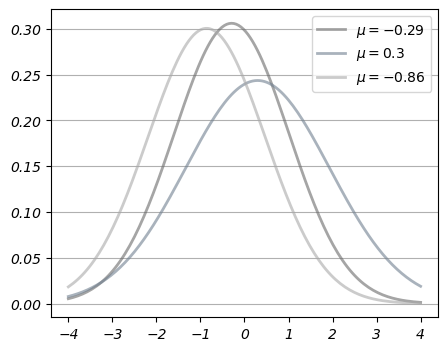
രണ്ടാമത്തെ method ഉപയോഗിച്ച് overlay ചെയ്ത നമ്മുടെ density lines-ന്റെ style മാറ്റാം:

from cycler import cycler

# set to the default style sheet
plt.style.use('default')

# You can update single values using keys:

# Set the font style to italic
plt.rcParams['font.style'] = 'italic'

# Update linewidth
plt.rcParams['lines.linewidth'] = 2


# You can also update many values at once using the update() method:

parameters = {

    # Change default figure size
    'figure.figsize': (5, 4),

    # Add horizontal grid lines
    'axes.grid': True,
    'axes.grid.axis': 'y',

    # Update colors for density lines
    'axes.prop_cycle': cycler('color', 
                            ['dimgray', 'slategrey', 'darkgray'])
}

plt.rcParams.update(parameters)

Note

ഈ settings global ആണ്.

.rcParams-ലെ parameters മാറ്റിയതിന് ശേഷം generate ചെയ്യുന്ന ഏതൊരു plot-നും ഈ setting affect ചെയ്യും.

fig, ax = plt.subplots()
x = np.linspace(-4, 4, 150)
for i in range(3):
    m, s = uniform(-1, 1), uniform(1, 2)
    y = norm.pdf(x, loc=m, scale=s)
    current_label = rf'$\mu = {m:.2}$'
    ax.plot(x, y, linewidth=2, alpha=0.6, label=current_label)
ax.legend()
plt.show()
_images/c8571102d4182a8bbb6efeba0a9c25e81a045de063f742a06b090d94a434bf54.png

നിങ്ങളുടെ style വീണ്ടും default ആയി മാറ്റാൻ default style sheet വീണ്ടും apply ചെയ്യുക:

plt.style.use('default')

# Reset default figure size
plt.rcParams['figure.figsize'] = (10, 6)

3.4. Further Reading#

  • Matplotlib gallery ധാരാളം examples provide ചെയ്യുന്നു.

  • Nicolas Rougier, Mike Muller, Gael Varoquaux എന്നിവരുടെ ഒരു നല്ല Matplotlib tutorial.

  • mpltools plot styles-ന് ഇടയിൽ എളുപ്പം switching ചെയ്യാൻ അനുവദിക്കുന്നു.

  • Seaborn Matplotlib-ൽ common ആയ statistics plots സഹായിക്കുന്നു.

3.5. Exercises#

Exercise 3.1

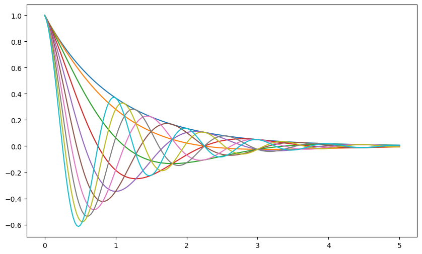
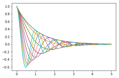
Plot the function

\[ f(x) = \cos(\pi \theta x) \exp(-x) \]

over the interval \([0, 5]\) for each \(\theta\) in np.linspace(0, 2, 10).

Place all the curves in the same figure.

The output should look like this
_images/matplotlib_ex1.png