6 Linear Decision Processes

In this chapter, we define linear decision processes (LDPs). In terms of level of generality, we can think of LDPs as sitting between MDPs, as discussed in Section 1.2, and the ADPs we considered in Chapter 2--Chapter 5:

with all inclusions being strict. LDPs have a range of advantages over MDPs while maintaining much of their tractability. One advantage is that we can work with state-dependent discounting, which is particularly important for economic and financial applications. Another is that their flexible structure makes them easy to apply. For example, optimal stopping problems can be embedded directly into the LDP framework, whereas embedding optimal stopping problems into MDPs requires expanding the state space.

LDPs differ from ADPs by including actions explicitly, instead of taking policy operators as the basic primitive. This is a more traditional perspective: one where controllers observe states and respond to those states by choosing actions. Ultimately, a choice of action given a state will take the form of a policy function; that will lead us back to the ADPs. By studying this circle, we can leverage theory from our earlier chapters.

LDPs are more limited than ADPs, but also more concrete and more structured. For example, they provide an algebraic formula for computing lifetime values similar to the one available for MDPs (see, e.g., (1.42) on page ). This formula is not available for general ADPs. Thus, for LDPs, the HPI step requiring computation of lifetime values from policies is fully articulated, at least at a theoretical level. Another advantage of LDPs, relative to ADPs, is that we can start to construct systematic conditions for regularity, or existence of greedy policies, unlike in previous chapters.

We begin with the theoretical foundations in Section 6.1. After introducing Feller properties in Section 6.1.1, we define LDPs in Section 6.1.2.1 and present optimality results. We then treat exogenous discount processes (Section 6.1.4) and specialize the LDP framework to MDPs on general state spaces (Section 6.1.5). In this chapter, we focus on the bounded case; unbounded models are handled in Chapter 7. Section 6.2.1 and Section 6.2.2 apply the theory to natural resource management and optimal savings with stochastic rates of return.

6.1Theory¶

In this section we develop the foundational theory of linear decision processes. We begin in Section 6.1.1 by studying Feller properties of transition kernels, which provide the continuity conditions needed for existence of optimal policies. We then define LDPs in Section 6.1.2.1, give examples, and discuss lifetime values. Next we present optimality results and their implications. Section 6.1.4 treats exogenous discount processes, and Section 6.1.5 specializes the LDP framework to Markov decision processes on general state spaces.

6.1.1Feller Properties¶

Since we are always interested in whether or not optimal policies exist, we study conditions under which future values are continuous in states and actions. In the case of LDPs, this continuity will require that integrals of transition kernels vary continuously with actions. (For background on transition kernels see Section A.5.4.1.) Here we provide a collection of definitions and results that help us address this question.

Throughout this section,

• $\Xsf$ and $\Asf$ are separable metric spaces,

• $\| \cdot \| \coloneq \| \cdot \|_\infty$ is the supremum norm,

• $\Gsf$ is a subset of $\Xsf \times \Asf$, and

• $K$ is a transition kernel mapping $b\Xsf$ to $b\Gsf$.

Here you can think of $\Gsf$ as a collection of feasible state-action pairs. The last statement means that

is in $b\Gsf$ whenever $v \in b\Xsf$.

Extending standard terminology, we will say that the transition kernel $K$ is

• weak Feller if $Kh$ is continuous on $\Gsf$ whenever $h \in b c\Xsf$ and

• strong Feller if $Kh$ is continuous on $\Gsf$ whenever $h \in b \Xsf$.

Let’s look at some special cases.

The strong Feller property requires more conditions, since we need to map a potentially discontinuous function $h$ into a continuous function $Kh$. For this, we rely on smoothing properties of the integral. To obtain these properties we introduce a “dominating” measure $\mu$ on $(\Xsf, \bB)$, which we assume to be $\sigma$-finite. A Borel measurable map $p$ from $\Gsf \times \Xsf$ to $\RR$ is called a density kernel from $\Gsf$ to $\Xsf$ with dominating measure $\mu$ if $p$ is nonnegative and

We say that a stochastic kernel $P$ from $\Gsf$ to $\Xsf$ has density kernel $p$ with dominating measure $\mu$ if $p$ is a density kernel on $\Xsf$ and

If the dominating measure $\mu$ is not identified in the discussion below then we will be referring to Lebesgue measure, and we write $\diff x$ instead of $\mu(\diff x)$. The following lemma shows how a continuous density kernel can transform discontinuous functions into continuous ones under integration.

6.1.2LDPs¶

We now introduce LDPs and study their basic properties. Section 6.1.2.1 defines LDPs and connects them to the ADP framework. We then present several examples, showing which models can and cannot be expressed as LDPs. Finally, we discuss lifetime values and their computation in the LDP setting.

6.1.2.1Definition¶

Let $\Xsf$ and $\Asf$ be separable metric spaces, referred to henceforth as the state and action spaces. As before, $\| \cdot \|$ denotes the supremum norm on $b \Xsf$. Given $\Xsf$ and $\Asf$, a linear decision process (LDP) is a tuple $(\Gamma, r, K)$ containing

1. a nonempty correspondence $\Gamma$ from $\Xsf$ to $\Asf$ called the feasible correspondence, with an associated set of feasible state-action pairs

2. a bounded Borel measurable reward function $r$ mapping $\Gsf$ into $\RR$, and

3. a transition kernel $K$ from $\Gsf$ to $\Xsf$ satisfying $Kv \in b\Gsf$ whenever $v \in b\Xsf$.

The set $\Gamma(x)$ represents all actions available to a controller in state $x$. Figure Figure 6.1 shows an illustration of one possible correspondence $\Gamma$ when $\Asf = \Xsf = \RR_+$, along with $\Gsf$, the resulting set of feasible state-action pairs. When representing the LDP by the tuple $(\Gamma, r, K)$, we are treating $\Xsf$ and $\Asf$ as understood from context.

For the LDP $(\Gamma, r, K)$, a feasible policy is a Borel measurable map $\sigma \colon \Xsf \to \Asf$ such that $\sigma(x) \in \Gamma(x)$ for all $x \in \Xsf$. Figure 6.2 shows a feasible policy $\sigma$ in the same setting.

We let $\Sigma$ denote the set of all feasible policies. With these policies in hand, we define the set of policy operators associated with $(\Gamma, r, K)$ via

where $v$ varies over $b \Xsf$.

The assumption that $\Xsf$ and $\Asf$ are metric spaces is important in some applications and irrelevant in others. For simplicity, we maintain it throughout. When $\Xsf$ and $\Asf$ are discrete, the metric in question is always understood to be the discrete metric. In this case, every subset of these sets is a Borel set, so the measurability constraint in the definition of $\Sigma$ never binds.

6.1.2.2ADP Representation¶

With

we can also write the policy operator (6.13) as

Given $v \in b \Xsf$, we have $Kv \in b\Gsf$ and hence $K_\sigma v \in b\Xsf$. Since $b \Xsf$ is a vector space, it follows that $T_\sigma \, v$ is in $b \Xsf$. Since $K$ is a transition kernel, $K_\sigma$ is a positive linear operator, so $T_\sigma$ is order preserving. Hence

is an ADP. We call $(V, \TT_{\rm LDP})$ the ADP generated by $(\Gamma, r, K)$ and use the following obvious conventions:

• $(\Gamma, r, K)$ is called well-posed (resp., regular, order stable, etc.) if $(V, \TT_{\rm LDP})$ is well-posed (resp., regular, order stable, etc.).

• $v_\sigma$ is the $\sigma$-value function for $(\Gamma, r, K)$ when $v_\sigma$ is the $\sigma$-value function for $(V, \TT_{\rm LDP})$,

• $\sigma$ is called optimal for $(\Gamma, r, K)$ when $\sigma$ is optimal for $(V, \TT_{\rm LDP})$,

• etc.

We notice that each $T_\sigma$ has the affine form from the ADP analysis in Section 4.1.2.3, with $K_\sigma \in \blop_+(b\Xsf)$ by Theorem A.5.25. We will use the theorems in that section for some of our optimality results.

6.1.2.3Examples¶

Let’s discuss some examples. Some but not all of these examples can be framed as LDPs.

6.1.2.4Lifetime Values¶

Let $(\Gamma, r, K)$ be an LDP with state space $\Xsf$, action space $\Asf$. Given a policy $\sigma \in \Sigma$, the $\sigma$-value function $v_\sigma$ is defined as the fixed point of the policy operator $T_\sigma$ in (6.13). As a result, $v_\sigma$ satisfies the recursion

If the spectral radius condition $\rho(K_\sigma) < 1$ holds, then, by the Neumann series lemma (see, in particular Corollary A.4.11 on page ), the operator $I - K_\sigma$ is invertible on $b \Xsf$ and the unique solution to (6.21) is

The $t$-th term $K_\sigma^t r_\sigma$ gives the expected reward at time $t$ under policy $\sigma$, discounted back to the present.

The explicit representation of $v_\sigma$ in (6.22) is valuable for computation. For example, the MDP version of HPI in Algorithm 1.2.2 can be extended to the current setting by replacing $v \leftarrow (I - \beta P_{\sigma} )^{-1} r_{\sigma}$ with $v \leftarrow (I - K_{\sigma} )^{-1} r_{\sigma}$. Under the conditions of Proposition 6.1.3, with $K$ strong Feller, this algorithm converges.

6.1.3Optimality Results¶

Now we turn to optimality results. We first treat the case where $\TT$ is finite, and then shift to general (metric) state and action spaces by adding continuity conditions. We conclude by deriving implications for greedy policies and the Bellman operator.

In the following, we suppose that $(\Gamma, r, K)$ is an LDP with state space $\Xsf$ and action space $\Asf$. As before, these sets are separable metric spaces (with the discrete topology when finite). As shown in Section 6.1.2.1, the LDP $(\Gamma, r, K)$ generates an ADP $(b\Xsf, \TT_{\rm LDP})$ where each $T_\sigma \in \TT_{\rm LDP}$ has the affine form $T_\sigma v = r_\sigma + K_\sigma v$. We will infer optimality of the LDP by studying this ADP.

6.1.3.1Results¶

First we present a result that works for the finite case.

To shift to the general case, we inject some continuity.

Recalling the definition of a discount operator from page , we can state the following result.

6.1.3.2Implications¶

Let $(\Gamma, r, K)$ be a given LDP. Clearly $\sigma \in \Sigma$ is $v$-greedy for $(\Gamma, r, K)$ if and only if

for all $\tau \in \Sigma$ and $x \in \Xsf$. The Bellman operator obeys

If, say, the conditions of Proposition 6.1.3 hold and $K$ is strong Feller, then, for every $v \in b \Xsf$, there always exists a $\sigma \in \Sigma$ obeying

(See the proof of Proposition 6.1.3.) In this setting, a policy $\sigma \in \Sigma$ is $v$-greedy if and only if (6.25) holds. Moreover, the Bellman operator simplifies to

for every $v \in b \Xsf$. These expressions remain valid in the weak Feller setting when we restrict to $v \in b c \Xsf$.

6.1.4Exogenous Discount Processes¶

In Chapter 4 we look at several settings that include state-dependent discounting. In each case the setting was relatively simple: either a binary stopping problem or a model with discrete states and actions. Here we’ll look at a problem with continuous state and action spaces. To make this setting tractable, we’ll insist that the discount factor process depends only on an exogenous state (i.e., a state that is not influenced by decisions of the agent).

6.1.4.1Discount Factor Processes¶

When the discount factor varies over time, forming a sequence $(\beta_t)_{t \geq 0}$, the present value of a random time $t$ payoff $H_t$ has the general form $\EE \, \beta_0 \cdots \beta_{t-1} H_t$. In this section we formalize this idea in a Markov environment and examine some simple consequences.

Let $\Zsf$ be a metric space and let $Q$ be a stochastic kernel on $\Zsf$. Let $(Z_t)$ be $Q$-Markov on $\Zsf$. Let $\beta \in b\Zsf$ be a nonnegative function and consider the discount factor process $(\beta_t)_{t \geq 0}$ where $\beta_t \coloneq \beta(Z_t)$ for all $t$. We introduce the operator

Our next lemma connects powers of $K_Q$ to expected present values.

We can confirm this rather natural expression by induction.

The next result follows from Gelfand’s formula for the spectral radius (p. ) and the details of the argument can be seen in Example 4.1.1.

Now consider pricing an infinite horizon cash flow $(h(Z_t))_{t \geq 0}$. We set

6.1.4.2An LDP with Exogenous Discounting¶

Let $\Xsf$ and $\Asf$ be separable metric spaces and let $(\Gamma, r, K)$ be an LDP with state space $\Xsf$ and action space $\Asf$. Suppose further that $\Xsf$ is a product space of the form $\Ysf \times \Zsf$ and that $K$ has the form

where

• $R$ is a stochastic kernel from $\Gsf$ to $\Ysf$,

• $Q$ is a stochastic kernel from $\Zsf$ to $\Zsf$, and

• $\beta$ is an element of $bc\Zsf$.

We call $R$ the endogenous kernel, $Q$ the exogenous kernel and $\beta$ the discount function. The expression for $K$ tells us that the endogenous state $y$ updates via the kernel $R$, depending on current state $x=(y,z)$ and action $a$, while $z$ updates via $Q$. Since we are taking products, the two updates are independent. The exogenous process feeds into values and hence optimal policies through its impact on the discount factor.

To make our lives slightly easier, we’ll assume that $\Zsf$ is finite. As with every other finite set, we endow $\Zsf$ with the discrete topology.

Let $K_Q$ be defined as in (6.27). In this setting, we have the following result.

6.1.5Markov Decision Processes¶

We treated discrete MDPs in Section 1.2. Let’s now consider MDPs on general state spaces. Mathematically, MDPs are LDPs with a fixed discount factor and Markov dynamics under any fixed policy. On one hand, MDPs are a special case of LDPs and need no separate theoretical discussion. On the other hand, MDPs are a benchmark representation of a dynamic program, used throughout mathematics, operations research, and computer science. For this reason we’ll take the time to specialize our LDP results to the Markov setting. Throughout this section, $\Xsf$ and $\Asf$ are separable metric spaces.

6.1.5.1Theory¶

Let $(\Gamma, r, K)$ be an LDP with state space $\Xsf$ and action space $\Asf$. This LDP is called a Markov Decision Process (MDP) when the transition kernel has the form

for some $\beta \in [0, 1)$ and some stochastic kernel $P$ from $\Gsf$ to $\Xsf$.

The MDP above will be represented by the tuple $(\Gamma, r, \beta, P)$. The ADP generated by this MDP will be denoted $(b\Xsf, \TT_{\rm MDP})$, where

Choosing a policy $\sigma$ picks out a stochastic kernel $P_\sigma$ on $\Xsf$, so choosing a policy is akin to picking an $\Xsf$-valued Markov process.

The following optimality result is an immediate consequence of Proposition 6.1.3.

6.1.5.2Implications¶

Since MDPs are such an important special case, we briefly specialize the implications from Section 6.1.2.1 to the MDP setting, replacing the general transition kernel $K$ with $\beta P$.

If the conditions of Proposition 6.1.7 hold and $P$ is strong Feller, then, for every $v \in b \Xsf$, there exists a $\sigma \in \Sigma$ obeying

and a policy $\sigma \in \Sigma$ is $v$-greedy if and only if (6.44) holds. Moreover, the Bellman operator simplifies to

for every $v \in b \Xsf$. These expressions remain valid without the strong Feller condition when we restrict to $v \in b c \Xsf$.

6.2Applications¶

We apply the theory developed above to two classes of problems. In Section 6.2.1 we study a natural resource management problem with state-dependent discounting. In Section 6.2.2 we analyze an optimal savings problem with stochastic rates of return on assets.

6.2.1Natural Resource Management¶

We consider a natural resource management application with Bellman equation

Here $y$ is the stock of the resource, $e$ is the current usage, $Q$ is a stochastic kernel on finite set $\Zsf$, $\phi$ is a distribution on $\RR_+$, $\pi \colon \RR_+ \to \RR$ is a profit function, $f \colon \RR_+ \to \RR_+$ is a transition function that updates the resource, $\beta \colon \Zsf \to \RR_+$ is a discount factor function, and $\xi$ is a multiplicative shock. The quantity $f(y-e) \xi$ is the next period stock.

If, say, $\xi$ is concentrated at 1 and $f(y-e) = y-e$, then this is exploitation of a nonrenewable resource. Another interpretation is that $y$ is a stock of fish at a given fishery, $e$ is current catch, $f$ is a transition rule that updates the stock given biological properties and environmental factors, and $\xi$ is a random shock to updating.

We assume that $\pi$ is continuous and bounded, and that the function $f$ is continuous. In the exogenous discounting setting of Section 6.1.4, the state is $\Xsf = \RR_+ \times \Zsf$, the action space is $\RR_+$, the feasible correspondence is $\Gamma(y, z) = [0, y]$, the reward function is $r(y, z, e) = \pi(e)$, and the transition kernel is

The endogenous kernel $R$ is determined by

The state evolves according to

where $\sigma$ is the optimal consumption policy. Let’s take a look at the kind of outcomes we can generate when $\beta$ is fixed, so that the exogenous shock process is degenerate. For simulation purposes, profits take the exponential form $\pi(x) = 1 - \exp(-\theta x^\gamma)$, while the transition function is set to $f(x) = x^\alpha \ell(x)$. Here $\ell$ is a generalized logistic function, while $\xi$ is lognormal.^[1] We compute the optimal policy $\sigma$ using value function iteration and then study the dynamics associated with the law of motion (6.49).

Figure 6.3 shows the optimal consumption policy $\sigma$ when $\beta = 0.96$, along with the 45 degree line, the map $y \mapsto f(y) \EE \xi$, which shows the expected next period stock with zero consumption, and the map $y \mapsto f(y - \sigma(y)) \EE \xi$, which shows expected dynamics under the optimal policy. Interestingly, the optimal choice for this parameterization is to consume none of the resource when the stock is small, enabling the stock to grow. Consumption only becomes positive when the stock is large enough to remain stable at a relatively high level. Of course, this kind of behavior will only be seen when the agent is sufficiently patient.

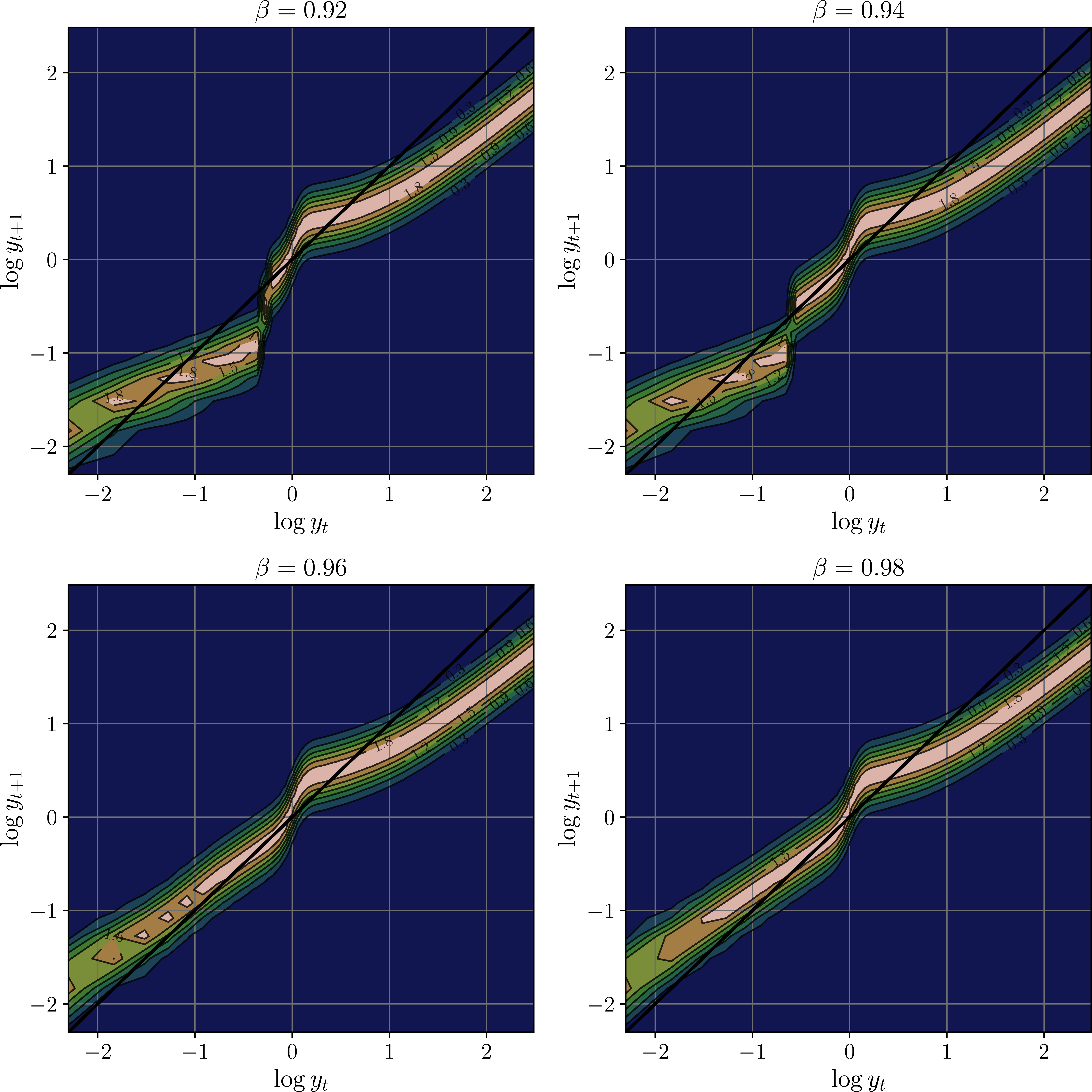
Figure 6.4 shows more detail on the dynamics by examining the stochastic kernel associated with the Markov dynamics in (6.49), after taking logs. Each stochastic kernel is represented as a contour plot of the relevant conditional density. The four subplots correspond to four different values of the discount factor $\beta$. For each value of $\beta$, the plot shows where probability mass for next period stock concentrates relative to current stock, given the associated optimal policy. Mass above the 45 degree line implies that the state moves up on average, while mass below indicates that the state drifts down.

As $\beta$ increases, the optimal policy adjusts to reduce current consumption and increase conservation, leading to probability mass shifting upward at each current state value. The changes in the stochastic kernel in Figure 6.4 seem minor but in fact they have large impacts on long run outcomes. Figure 6.5 illustrates this by showing an estimate of the stationary distribution corresponding to each Markov process. Densities were estimated by simulating 100 independent paths of length $1{,}000$ from a common initial condition. The plots show a sharp transition around $\beta=0.95$. For $\beta$ around that level, the long run stock is low. For slightly higher $\beta$, the optimal path leads to much larger stocks (recalling that we are working in logs).

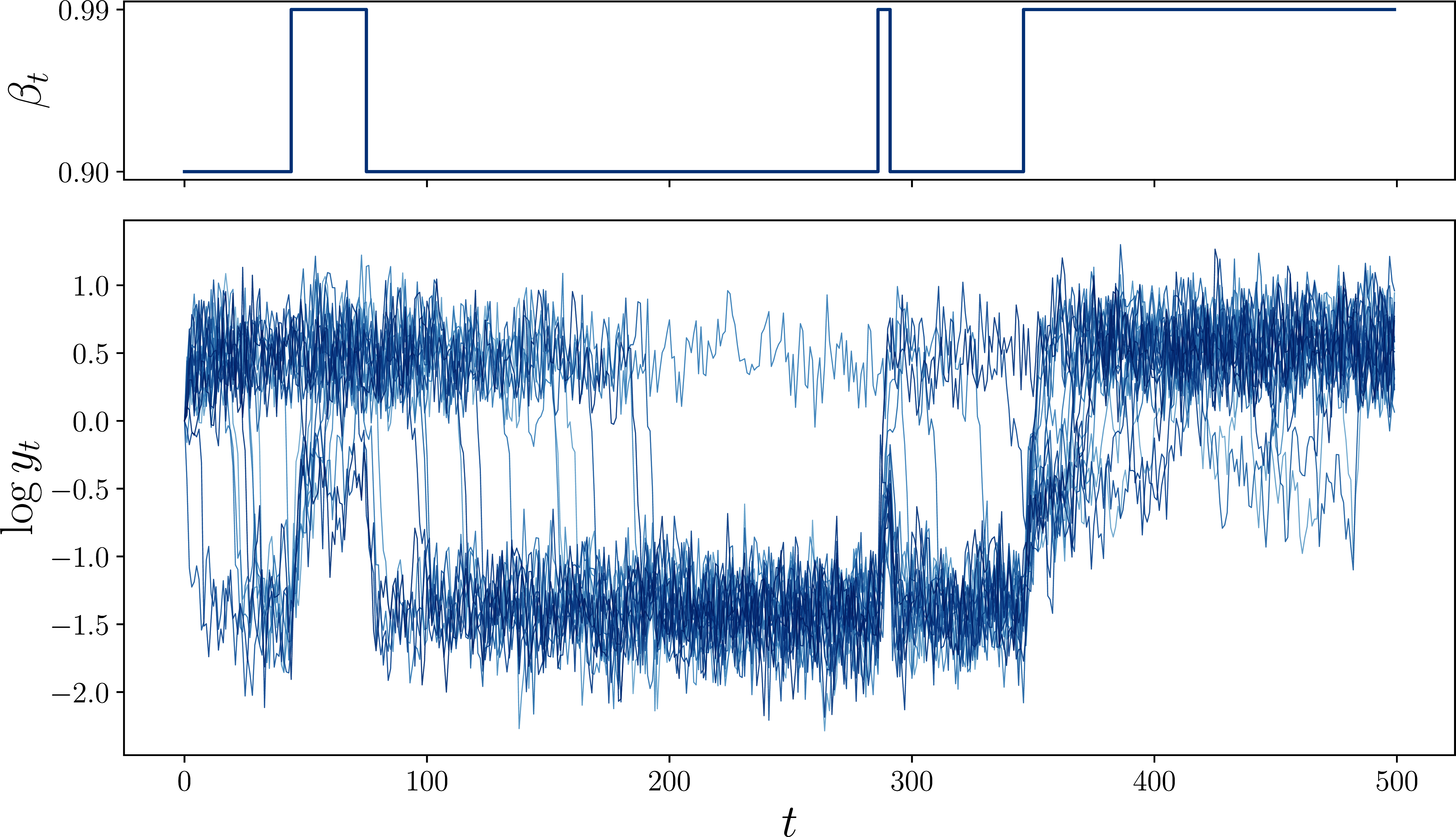
Up until now we’ve taken $\beta$ as a fixed parameter when computing optimal policies. Now we allow it to vary with an exogenous state $z$ via $\beta(z)$, in line with our theoretical analysis in Proposition 6.2.1. To illustrate the effect of state-dependent discounting, we set $\Zsf = \{0.9, 0.99\}$ and $\beta(z) = z$. The exogenous state follows a two-state Markov chain with persistence 0.99 in each state. Other model parameters are as in the fixed-$\beta$ experiments above. We computed optimal policies via value function iteration on the product space $\RR_+ \times \Zsf$.

Figure 6.7 shows the outcome of simulating 20 independent paths of the resource stock under the optimal policy, given a single realization of the exogenous process $(Z_t)$. The top panel displays the discount factor $\beta_t$, while the bottom panel shows the corresponding log stock $\log y_t$ over multiple alternative paths for $(\xi_t)$. During patient regimes, the stock tends to grow as the optimal policy shifts toward conservation. When the discount factor drops, the agent increases exploitation and the stock tends to decline.

6.2.2Stochastic Rates of Return¶

As our next application, we consider a savings problem with a persistent state process and a stochastic rate of return on assets. Stochastic returns on assets appear to be important in generating sufficiently heavy right tails in wealth distributions when we take models to the data.

In this model,

• the state is $x = (w, z)$, where $w \in \RR_+$ is wealth and $z$ is an exogenous state process on finite set $\Zsf$ with stochastic kernel (matrix) $Q$,

• the action $a$ is current consumption $c$, taking values in $\RR_+$,

• the feasible correspondence is $\Gamma(x) = \Gamma(w, z) = [0, w]$,

• the reward is $r(x, a) = r((w, z), c) = u(c)$, where $u$ is bounded and continuous,

• the discount factor is $\beta \in (0,1)$, and

• the stochastic kernel takes the form

The kernel can be explained as follows: Labor income is affected by an iid shock $s'$ drawn from distribution $\phi \in \dD(\Ssf)$, where $\Ssf$ is a topological space. In addition, both the interest rate and labor income are impacted by a common persistent component $z$. The latter is driven by stochastic matrix $Q$. We give $\Zsf$ the discrete topology and $\Xsf = \RR_+ \times \Zsf$ the product topology.

We apply Proposition 6.1.7 to this model. For Assumption 6.1.1, continuity and compact-valuedness of $\Gamma$ follow from Exercise A.20, and $r = u$ is continuous by assumption. It remains to verify that $P$ is weak Feller. Fixing $v \in bc\Xsf$, we must show that the mapping

is continuous on $\Gsf$. Taking $(w_n, z_n, c_n) \to (w, z, c)$ in $\Gsf$, since $\Zsf$ has the discrete topology, $(z_n)$ is eventually constant at $z$. Hence it suffices to show that $m(w_n, z, c_n) \to m(w, z, c)$. This follows from continuity and boundedness of $v$ and the dominated convergence theorem.

Hence Proposition 6.1.7 applies and the conclusions therein hold. The Bellman operator takes the form

6.3Chapter Notes¶

The Feller properties discussed in Section 6.1.1 are standard tools in the theory of Markov chains and stochastic processes. For further background, see Hernández-Lerma & Lasserre (2012) or Bäuerle & Rieder (2011). The use of Feller conditions to guarantee existence of optimal policies in MDPs and dynamic programs dates back to the foundational work of Blackwell (1965). Scheffé’s lemma, used in the proof of Lemma 6.1.1, is a classical result in measure theory (see p. ).

Standard proofs of the optimality results we stated for MDPs on general state spaces (Section 6.1.5) can be found in Puterman (2005), Bäuerle & Rieder (2011), Hernández-Lerma & Lasserre (2012), Stachurski (2022), or Sargent & Stachurski (2025).

The exposition of exogenous discount processes in Section 6.1.4 is partly based on Stachurski & Zhang (2021). State-dependent discounting in the context of dynamic programming is also studied in Jaśkiewicz et al. (2014).

The natural resource management model in Section 6.2.1 is a standard bioeconomic exploitation model; see Clark (2010) for background. Versions with state-dependent discounting are relevant for modeling resource management under fluctuating economic conditions.

For a discussion of stochastic rates of return on financial income, as considered in Section 6.2.2, see Benhabib et al. (2015) or Stachurski & Toda (2019). The latter shows that heavy-tailed wealth distributions can also be generated by time preference shocks, but this channel is relatively unrealistic, since it requires that all households in the economy simultaneously experience time preference shocks in the same direction. Additional work on the relationship between stochastic discount factors and wealth distributions includes Toda (2019), Ma et al. (2020), and Nirei & Aoki (2015).

What we have called linear decision processes (LDPs) might be confused with Markov decision processes having linear reward or cost functions. The latter are a special case of the former. For a recent discussion of MDPs with linear cost functions, see Rantzer (2022) and Li & Bertsekas (2024).