In this chapter we study what Sargent & Stachurski (2025) call recursive decision processes (RDPs). The following display shows where RDPs fit relative to the other major classes of DP models studied so far in this book:
MDPs ⊂ LDPs ⊂ RDPs ⊂ ADPs.
The main role of RDPs is to extend LDPs by accommodating nonlinearities in aggregators and calculation of present values. Another difference between this chapter and our discussion of LDPs is that we allow for unbounded rewards and value functions. While this can also be done in an LDP setting, the corresponding analysis turns out to be cleaner when working with RDPs.
Section 7.1 introduces the RDP framework, provides examples, clarifies the relationships between RDPs, LDPs and ADPs, and discusses existence of greedy policies. Section 7.2.1 and Section 7.2.2 present optimality results—first for bounded rewards and then for unbounded rewards handled via weighted contractions—while Section 7.2.3 gives conditions under which the value function is monotone, concave, or uniquely determined. After a digression on certainty equivalents (Section 7.2.4), we extend the optimality theory to MDPs with general certainty equivalents (Section 7.2.5). Section 7.3.1 applies the theory to optimal savings with unbounded utility, and we then study irreversible investment under risk neutrality, risk aversion, and ambiguity aversion.
Section 7.1.1 defines RDPs and provides examples. We then clarify the relationships between RDPs, LDPs and ADPs, and discuss existence of greedy policies in Section 7.1.3.
for some suitable choice of B. Here x is the state, a is an action, Γ is a feasible correspondence and B is an “aggregator,” with interpretation
B(x,a,v)= total lifetime rewards, contingent on current action a, current state x and the use of v to evaluate future states.
In Section 7.1.1.1–Section 7.1.1.5 we improve this definition and then provide examples. As usual, in a topological space setting, “measurable” means “Borel measurable” unless otherwise stated.
Let X and A be separable metric spaces, referred to henceforth as the state and action spaces respectively. Given these spaces, a recursive decision process (RDP) is a tuple (Γ,V,B) containing
a nonempty correspondence Γ from X to A called the feasible correspondence, with an associated set of feasible state-action pairs
G:=graphΓ={(x,a)∈X×A:a∈Γ(x)}
and an associated set of feasible policies
Σ:={all measurable σ:X→A satisfying σ(x)∈Γ(x) for all x∈X},
a subset V of RX called the value space,
a map B:G×V→R, referred to as an aggregator, satisfying the monotonicity condition
Several objects, such as X,A and Γ are familiar from our definition of LDPs in Section 6.1.2.1. Analgous to the LDP case, when representing the RDP by the tuple (Γ,V,B), we are treating X and A as understood from context.
The value space V is a class of functions that assign values to states. The order on the left side of (7.2) is the usual pointwise partial order for functions. The monotonicity restriction is natural: relative to v, if rewards are at least as high under w in every future state, then the total rewards we can extract under w should be at least as high.
The final condition, in (7.3), is a consistency condition implying that V is large enough to capture the value of following a particular policy.
In Section 1.2 we introduced the basic MDP model, with finite state space X, finite action space A, and remaining primitives (Γ,r,β,P) as given in Section 1.2.1.1. This maps easily to the RDP setting by taking V=RX, Γ as given, and
B(x,a,v)=r(x,a)+βx′∑v(x′)P(x,a,x′)
for (x,a)∈G and v∈RX.
For this model, it is clear that the RDP Bellman equation v(x)=maxa∈Γ(x)B(x,a,v) from (7.1) agrees with the original expression we gave in (1.20).
Recall the firm decision problem we analyzed in Section 1.1.1.2, where the decision is binary (0 means continue and 1 means sell) and the state x takes values in a set X and evolves via stochastic kernel P. To map this problem to an RDP we set A={0,1} and Γ(x)=A for all x. We take V:=bX as the value space and set
The monotonicity condition (7.2) clearly holds. A policy is a B-measurable map σ:X→{0,1}. Given any such policy and any v∈bX, the function
m(x):=σ(x)s+(1−σ(x))[π(x)+β∫v(x′)P(x,dx′)]
is in bX (since π is assumed to be bounded), so the consistency condition (7.3) also holds. For this model, the RDP Bellman equation v(x)=maxa∈Γ(x)B(x,a,v) becomes
v(x)=a∈{0,1}max{as+(1−a)[π(x)+β∫v(x′)P(x,dx′)]}
This is equivalent to the original statement of the Bellman equation in Theorem 1.1.1.
The firm valuation problem can also fit into the RDP framework when profits are unbounded, at least in some cases. For example, suppose that X=R+, that ℓ is a given weight function on R+ (see Section A.5.3.5), and that there exist nonnegative constants α,η,δ such that
(These conditions bound the rate at which profits grow.) We again take B as in (7.4) and Γ(x)={0,1} for all x∈R+. We set V equal to bℓX, the set of measurable functions v∈RX with ∥v∥ℓ<∞. (Here ∥⋅∥ℓ denotes the ℓ-weighted supremum norm, as in Section A.5.3.5.)
Consider the optimal savings problem studied in Section 1.3. The state is w∈R+ and the action is c∈R+. The feasible correspondence is Γ(w)=[0,w] and V:=bR+ is the value space. We set
B(w,c,v)=u(c)+β∫v(R(w−c)+y)ϕ(dy)(v∈V,0⩽c⩽w).
As in Assumption 1.3.1, we take u to be bounded and continuous. Under these restrictions, the tuple (Γ,V,B) is an RDP. The function B is real-valued and the monotonicity condition (7.2) clearly holds. The consistency condition (7.3) holds because, by the definition of Γ, a policy is a Borel measurable map σ:R+→R+ with 0⩽σ(w)⩽w for all w, and given any such policy and any v∈bR+, the function
m(w):=u(σ(w))+β∫v(R(w−σ(w))+y)ϕ(dy)
is measurable and bounded (since u is bounded and continuous).
For this model, the RDP Bellman equation v(x)=maxa∈Γ(x)B(x,a,v) from (7.1) agrees with the optimal savings Bellman equation in (1.52).
7.1.1.6Example: Savings with Kreps–Porteus Expectations¶
Consider a variation of the optimal savings model from Section 7.1.1.5 with Epstein–Zin-type preferences. To simplify the presentation, we set the EIS parameter to ψ=∞, so that the CES aggregator reduces to addition, while retaining the nonlinear Kreps–Porteus expectation over future values. The Bellman equation becomes
where γ>0 with γ=1 is the coefficient of relative risk aversion.
As before, the state is w∈R+, the action is c∈R+, and Γ(w)=[0,w]. To avoid raising zero to a negative power, we assume that u is measurable and that there exist constants 0<u⩽uˉ<∞ with u⩽u(c)⩽uˉ for all c∈R+. The aggregator is
B(w,c,v)=(1−β)u(c)+β(∫v(R(w−c)+y)1−γϕ(dy))1−γ1.
We set the value space V to be all measurable functions v:R+→[u,uˉ].
With B defined as above, the RDP Bellman equation v(x)=maxa∈Γ(x)B(x,a,v) from (7.1) agrees with (7.6).
Here r maps G×X to R and other primitives are unchanged. We take V=RX, Γ as given, and set
B(x,a,v)=x′∑{r(x,a,x′)+βv(x′)}P(x,a,x′)
Evidently, for the associated RDP (Γ,V,B), the monotonicity and consistency conditions (7.2) and (7.3) both hold. For this choice of B, the RDP Bellman equation v(x)=maxa∈Γ(x)B(x,a,v) agrees with the modified MDP Bellman equation in (7.7).
In §Example 6.1.6 we discussed a risk-sensitive MDP with entropic certainty equivalent. This model can be embedded in the RDP framework by setting V=RX, Γ as given, and
As mentioned at the start of the chapter, we have MDPs ⊂ LDPs ⊂ RDPs ⊂ ADPs and the inclusions are all strict. We already know that the first inclusion is strict (consider, for example, the LDP with state-dependent discounting in Section 6.1.4). Here we review the remaining relationships.
the resulting tuple (Γ,V,B) is an RDP. To see this, note that V=bX is a subset of RX, so we only need to check the monotonicity and consistency conditions for the aggregator B. For monotonicity, fix (x,a)∈G and v,w∈V with v⩽w. Since K(x,a,⋅) is a nonnegative measure, we have ∫v(x′)K(x,a,dx′)⩽∫w(x′)K(x,a,dx′) and hence B(x,a,v)⩽B(x,a,w). For consistency, fix σ∈Σ and v∈bX. We need to show that m(x):=B(x,σ(x),v) is in bX. This follows from the LDP conditions, which require r∈bG and Kv∈bG whenever v∈bX.
The risk-sensitive MDP in Section 7.1.1.8 is an RDP but not an LDP, since the aggregator is nonlinear in future values.
Every RDP generates an ADP. To see this, let (Γ,V,B) be an RDP with state space X and action space A. The set V is paired with the pointwise partial order. With Σ as the set of feasible policies and given σ in Σ, we define Tσ by
(Tσv)(x)=B(x,σ(x),v)(x∈X,v∈V).
The monotonicity and consistency conditions in (7.2)–(7.3) imply that Tσ is an order-preserving self-map on V. Hence, with T as the set of all policy operators, the pair (V,T) is an ADP. We call (V,T) the ADP generated by (Γ,V,B).
For ADPs generated by RDPs, we can provide intuitive representations of greedy policies and the Bellman equation. For example, we recall from our ADP definition in (2.1) that a policy σ∈Σ is v-greedy for ADP (V,T) if Tτv⩽Tσv for all τ∈Σ. If (V,T) is generated by (Γ,V,B), then this is equivalent to the statement that
Also, we recall that the ADP Bellman operator is defined by Tv=⋁σTσv whenever the supremum exists. When (V,T) is generated by (Γ,V,B), this is equivalent to the statement (Tv)(x)=supσ∈ΣB(x,σ(x),v) for all x∈X whenever the pointwise supremum exists (see Exercise A.1.4). Under reasonable conditions on Γ and B, we will show that this can be improved to the stronger form
Since every RDP is an ADP, we can use ADP optimality results to study RDPs. Given an RDP (Γ,V,B) and its generated ADP (V,T), we make the obvious connections, saying that
(Γ,V,B) is regular if (V,T) is regular,
T is the Bellman operator for (Γ,V,B) when T is the Bellman operator for (V,T),
σ is optimal for (Γ,V,B) when σ is optimal for (V,T),
Although the RDP framework is broad, there are significant dynamic programs that fall outside this framework.
In the examples above, it is possible to rearrange the problem so that the max operator is shifted to the outside and, thereby, construct a version that fits the RDP framework. But there are good reasons to avoid this, related to smoothness and dimensionality (see, e.g., Kristensen et al. (2021) or Rust (1994)).
As always, existence of greedy policies is important for our analysis. In this section, we investigate RDP environments where greedy policies exist. We begin with finite action spaces and then move to the general case.
We begin with the discrete choice setting, where greedy policies always exist.
Note that, in the simple setting of Lemma 7.1.1, the Bellman equation takes the form of (7.1). Below we investigate more complex settings where this is still true.
Let’s put together some sufficient conditions for optimality of RDP models. We will focus here on models that are naturally contracting. This permits us to handle dynamic programs with both bounded and unbounded rewards.
We begin in Section 7.2.1 with the bounded case, where the aggregator B is bounded and satisfies a Blackwell-type discounting condition. In Section 7.2.2 we extend to potentially unbounded rewards using weighted contractions. Finally, Section 7.2.3 investigates properties of solutions, giving sufficient conditions for the value function to be monotone, concave, or uniquely determined, and for the optimal policy to be continuous.
RDPs have strong optimality properties when they uniformly contract values. The current section investigates this case. Throughout this section, we assume that values are bounded. This typically occurs when reward functions are bounded. Later, in Section 7.2.2, we will consider unbounded settings.
Let X,A be separable metric spaces, let Γ be a nonempty correspondence from X to A, and let G be the feasible state-action pairs (see Section 7.1.1.1). Set V=bX. Let B:G×V→R be a given function such that
(x,a)↦B(x,a,v) is measurable on G for all v∈V, and
B(x,a,w)⩽B(x,a,v) for all w⩽v in V and (x,a)∈G.
The tuple (Γ,V,B) is an RDP. To see this, note that the monotonicity condition (7.2) is given by the second restriction on B above. For the consistency condition (7.3), fix σ∈Σ and v∈V. The function x↦B(x,σ(x),v) is measurable, since σ is measurable and (x,a)↦B(x,a,v) is measurable on G, and bounded, since B is bounded by Assumption 7.2.1. Hence B(⋅,σ(⋅),v)∈bX=V.
We seek optimality results for the RDP (Γ,V,B) introduced in Section 7.2.1.1. The simplest case is when the choice set is always finite. Also note that, in this setting, a policy σ is v-greedy if and only if (7.16) holds.
We now drop the finiteness assumption, while continuing to work with the RDP (Γ,V,B) introduced in Section 7.2.1.1. In place of finiteness, we consider two continuity conditions on B.
In Section 7.2.1, we considered RDPs that are both contracting and bounded. Some useful RDPs fail to have this boundedness property. Here we extend our results to potentially unbounded problems that still retain contractivity. (While the results obtained in Section 7.2.1 are special cases of the results presented here (after minor modifications), we decided to present them separately in order to provide simple sufficient conditions in the bounded case.)
When maximizing, the theory works best for problems where rewards are unbounded above and bounded below. (One approach to the reverse type of unboundedness can be found in Ma et al. (2022).) Because we focus on such problems, we will typically assume that rewards are nonnegative. This costs no generality in such settings, since optimal policies are invariant to additive shifts.
Throughout this section, ℓ is a weight function on X, ∥⋅∥ℓ denotes the ℓ-weighted supremum norm, and bℓX is all f:X→R with f/ℓ∈bX. See Section A.5.3.5 for background and discussion of weight functions and the space bℓX.
Let Γ be a nonempty correspondence from X to A and let G be the feasible state-action pairs (see Section 7.1.1.1). Set V=bℓX+, so that V is the nonnegative functions in bℓX. Let B:G×V→R+ be a given function. (In the current setting, where B can be unbounded, we restrict attention to the case where B is nonnegative. Since the weighted contraction approach pursued here works best for rewards that are unbounded above but bounded below, imposing nonnegativity costs very little in the way of generality.)
We suppose that
(x,a)↦B(x,a,v) is measurable on G for all v∈V, and
B(x,a,w)⩽B(x,a,v) for all w⩽v in V and (x,a)∈G.
We also require two conditions related to contractivity and ℓ-boundedness:
In this section, we seek sufficient conditions for the value and policy functions to have useful shape and continuity properties. We adopt the setting of Proposition 7.2.5 and study the properties of the RDP (Γ,V,B) discussed in that result. In the proofs below, we repeatedly use Lemma A.2.6.
First, we seek conditions under which the value function is increasing. In addition to the conditions in Proposition 7.2.5, we suppose that X is partially ordered by ⪯. Let
ibℓcX+:= the set of increasing functions in bℓcX+.
Both conditions in Assumption 7.2.8 are monotonicity conditions. The first is equivalent to stating that Γ is order preserving when viewed as a map from (X,⪯) to (℘(A),⊂). Here ℘(A) is the set of all subsets of A and ⊂ is the partial order induced by set inclusion (Example A.1.2).
Next we seek sufficient conditions for the value function to be concave. In this section, we assume that both X and A are convex subsets of a vector space.
The convexity requirement on G in Assumption 7.2.9 is equivalent to the statement that, for all x,x′ in X, all a∈Γ(x) all a′∈Γ(x′) and all λ∈[0,1], we have
λa+(1−λ)a′∈Γ(λx+(1−λ)x′).
By taking x=x′, we see that each set Γ(x) is convex in A.
When the conditions of Proposition 7.2.5 are in force, we know that at least one optimal policy exists in Σ. The question we ask now is, when is it unique? Not surprisingly, uniqueness can be obtained with a form of strict concavity.
Before continuing with the theory of RDPs, it will be helpful to review risk measures and certainty equivalents. These concepts are in one-to-one correspondence: we convert between them by flipping signs. Certainty equivalents can be understood as extensions of mathematical expectation that include attitudes towards risk. In later sections, we will tie the discussion of risk measures and certainty equivalents back into RDP theory and its applications.
(The existence of parallel literatures on risk measures and certainty equivalents reflects the fact that researchers in finance and engineering often think about minimizing risk, while economists typically concern themselves with maximizing rewards.[1] In this book, we tend to work with certainty equivalents, although the following discussion will allow readers to translate between the two.)
Throughout the following discussion, the triple (Ω,F,P) is a probability space and L∞:=L∞(Ω,F,P) is the set of essentially bounded random variables on (Ω,F,P); that is, all random Z admitting an N∈N with ∣Z∣⩽NP-a.s.
In this setting, a risk measure is a map R:L∞→R satisfying
(R1) Monotonicity: If Z,Z′∈L∞ and Z⩽Z′P-a.s., then R(Z′)⩽R(Z).
(R2) Cash invariance: R(Z+a)=R(Z)−a for all Z∈L∞ and a∈R.
A certainty equivalent is a map E:L∞→R satisfying
(C1) Monotonicity: If Z,Z′∈L∞ and Z⩽Z′P-a.s., then E(Z)⩽E(Z′).
(C2) Cash invariance: E(Z+a)=E(Z)+a for all Z∈L∞ and a∈R.
(Note that the meaning of monotonicity and cash invariance changes from R to E.)
We now define several significant subclasses of risk measures and state the corresponding properties of the associated certainty equivalent E=−R.
A risk measure R is called convex if
R(λZ+(1−λ)Z′)⩽λR(Z)+(1−λ)R(Z′)
for all Z,Z′∈L∞ and λ∈[0,1]. Obviously, R is convex if its negation E:=−R is concave:
E(λZ+(1−λ)Z′)⩾λE(Z)+(1−λ)E(Z′).
Concavity of E captures the idea that diversification is weakly preferred.
A risk measure R is called coherent if it is convex and positively homogeneous, meaning that R(λZ)=λR(Z) for all Z∈L∞ and λ>0. The certainty equivalent E=−R is then concave and positively homogeneous. Together with concavity, this means E is superadditive and positively homogeneous.
There is a dual representation theorem for convex risk measures, originally due to Föllmer & Schied (2002), that helps us interpret and manipulate these functionals. Here we restate their result in terms of concave certainty equivalents. In doing so, we will restrict attention to the law invariant case; that is, the case where E(Z) depends only on the distribution of Z for all Z∈L∞.[2]
In the theorem statement, PZ is P∘Z−1, the distribution of Z, and the infimum is over all Q∈P(R) such that Q is absolutely continuous with respect to PZ. The constraint Q≪PZ means that if PZ says an event is impossible, then Q must also say it’s impossible.
One way to interpret (7.20) is in terms of an adversarial agent who chooses Q to minimize the expected return EQ[Z], while being constrained by a penalty term α(Q). This is the robust optimization point of view: the agent makes choices that are robust to variations by a real or fictitious adversary. The penalty function α controls how far the adversary is able to deviate from the reference model PZ. From this perspective, the absolute continuity condition Q≪PZ means that the adversary is allowed to disagree about how likely different scenarios are, but not about which scenarios are conceivable.
A second interpretation involves ambiguity. The agent does not know the true model and PZ is only a reference point. The agent’s cautious reasoning forces him to entertain a range of plausible models. The penalty term α(Q) reflects how implausible Q is relative to PZ. The absolute continuity constraint defines what the agent considers to be possible—the set of scenarios that could actually occur.
Let’s look at examples, focusing primarily on certainty equivalents. Throughout this discussion, Z is an element of L∞, PZ is its distribution, FZ is its CDF, and FZ−1 is the inverse CDF.
The simplest certainty equivalent is mathematical expectation: E(Z)=E[Z]. This corresponds to risk neutrality: the agent is indifferent between any random variable and its mean. The other extreme is the pessimistic certainty equivalent
Ep(Z):=essinfZ=sup{a∈R:P{Z<a}=0}.
We can think of Ep(Z) as the left-hand end point of the support of Z. For the pessimistic certainty equivalent, the dual representation (7.20) becomes
Ep(Z)=Q≪PZinfEQ[Z],
Both of these examples are coherent.
Another example is the α-quantile certainty equivalent
Qα(Z)=FZ−1(α),α∈(0,1).
The value Qα(Z) is the α-quantile of Z. The corresponding risk measure Rα=−Qα is just α-level value-at-risk (VaR).
VaR admits some pathologies. For example, VaR is not convex, and hence can increase under diversification. These deficiencies have motivated the introduction of conditional value at risk (CVaR) (also called average value at risk, or expected shortfall), defined as
Rα(Z)=−α1∫0αFZ−1(t)dtα∈(0,1],
The corresponding CVaR certainty equivalent is Eα(Z)=−Rα(Z), interpreted as the mean of the α-tail of the distribution of Z---the average over the worst α-fraction of outcomes. The CVaR certainty equivalent is coherent and admits the dual representation
Eα(Z)=inf{EQ[Z]:Q≪PZ,dPZdQ⩽α1}.
The parameter α interpolates between the two previous cases:
α=1⟹E1(Z)=E[Z],α→0⟹Eα(Z)→essinfZ.
Another important case, already discussed in Chapter 1, is the entropic certainty equivalent
where DKL(Q∥PZ)=EQ[logdPZdQ] is the Kullback–Leibler divergence. The parameter γ controls the degree of risk aversion and interpolates between risk neutrality and worst case. In particular, γ→0 implies Eγ(Z)→E[Z], while γ→∞ implies Eγ(Z)→essinfZ.
It is worth noting here that the Kreps–Porteus expectation K(Z):=(E[Z1−γ])1/(1−γ) is not a certainty equivalent, at least according to our definition. While monotonicity holds, K fails cash invariance. This is, in essence, why Bellman and policy operators based around Epstein–Zin preferences often fail to be contractions. We discuss Kreps–Porteus expectations again in Section 7.3.4.
Let E be a certainty equivalent on L∞=L∞(Ω,F,P). We call Econtinuous if, given any uniformly bounded sequence (Zn)n∈N in L∞ and any Z∈L∞, we have
E(Zn)→E(Z)whenever Zn→ZP-almost surely.
In the definition above, uniform boundedness means that there exists an M<∞ with ∣Zn∣⩽M almost surely for all n. Continuity will be useful for the optimality theory developed below.
We first set up a standard MDP framework with aggregator based on mathematical expectation and then replace the expectation with a general certainty equivalent, showing that the fundamental optimality results carry over when the certainty equivalent is continuous.
We begin by setting up a basic MDP framework that can then be adapted to add risk preferences. To this end, let X and A be arbitrary metric spaces and let Γ be a nonempty correspondence from X to A. Let G={(x,a)∈X×A:a∈Γ(x)}. Consider an RDP with feasible correspondence Γ and aggregator
Here ξ is a random element that takes values in a metric space Z and has distribution ϕ, f is a measurable function from G×Z to X, and r is a measurable function from G to R. The discount factor β obeys 0⩽β<1. The value space is set to bX.
We can treat optimality and convergence of algorithms for the associated RDP (Γ,bX,B) using Proposition 6.1.7 from Chapter 6. Here, however, we’ll extend the model to use arbitrary certainty equivalents in place of E. Results for E will be a special case. The next section gives details.
Let’s consider replacing the expectation in (7.23), which corresponds to risk-neutrality over continuation values, with an arbitrary certainty equivalent E. The aggregator is now
Other primitives are left unchanged. The value space continues to be bX. We assume throughout that (x,a)↦E[v(f(x,a,ξ))] is measurable on G. We consider the RDP (Γ,bX,BE).
We now apply the RDP optimality theory developed in Section 7.2 to a range of dynamic programming problems. In Section 7.3.1 we revisit the optimal savings problem, this time with utility unbounded above, and verify the conditions of our weighted contraction results. We then study irreversible investment under risk neutrality (Section 7.3.2.1), risk aversion (Section 7.3.2.2), and ambiguity aversion (Section 7.3.3).
7.3.1Optimal Savings with Utility Unbounded Above¶
Here we again consider the optimal savings model from Section 1.3, but without the boundedness restriction on u. In particular, we assume that u is continuous, nonnegative, and increasing, and that
for some δ∈(β,1). Here (W^t) is defined recursively via W^t+1=RW^t+Yt+1 with W^0=w and (Yt)∼ iid ϕ. We can think of (W^t) as an upper bound process for wealth, achieved when consumption is always zero. As before, ϕ is a continuous density on R+. Our aim is to provide conditions under which the conclusions of Proposition 7.2.5 apply.
We set V=bℓR+, Γ(w)=[0,w], and
B(w,c,v)=u(c)+β∫v(R(w−c)+y)ϕ(dy).
The results above imply that Assumption 7.2.7 and Assumption 7.2.4 both hold. As a result, the conclusions of Proposition 7.2.5 apply. For example, the value function v∗ exists, is an element of bℓcR+, and satisfies
v∗(w)=0⩽c⩽wmax{u(c)+β∫v∗(R(w−c)+y)ϕ(dy)}
for all w⩾0. Moreover, VFI, OPI, and HPI all converge.
In general, OPI and VFI are the easiest to implement. Figure 7.1 illustrates the runtime of OPI as a function of m for this model with CRRA utility u(c)=(c1−γ−1)/(1−γ) and γ=0.5. The runtime of VFI is shown as a horizontal line. Since VFI is the special case of OPI with m=1, the leftmost point of the OPI curve coincides with the VFI runtime. The minimum is attained near m=40, where OPI runs roughly six times faster than VFI. Runtime then rises linearly in m. The key message is that OPI dominates VFI over a wide range of m.
Figure 7.1:Runtime of OPI vs. VFI for the optimal savings model
We begin with the risk-neutral case in Section 7.3.2.1, where standard contraction arguments apply. In Section 7.3.2.2 we introduce risk aversion by replacing mathematical expectation with a certainty equivalent, using the framework developed in Section 7.2.4.
Here k∈R+ is capital stock, i∈R+ is investment, β∈(0,1) is the discount factor, δ∈(0,1) is a depreciation rate, f is a production function, and z∈Rm is an exogenous state vector. The feasible correspondence is defined by Γ(k,z)=[0,θf(k,z)], where θ>0 is a borrowing constraint parameter. The state process evolves according to
Zt+1=g(Zt,ξt+1),(ξt)t⩾0∼ iid ϕ.
Each ξt takes values in a metric space Z, the distribution ϕ is an element of P(Z), and g:Rm×Z→Rm.
Some comments are in order. First, to simplify the presentation, we’ve set the output price to unity, so that f(k,z) is both output and revenue. This can easily be modified. Second, the boundedness restriction on f is not automatically satisfied in many cases but greatly simplifies the analysis. In terms of quantitative applications, the cost is not large. For example, f(k,z)=zkα can be replaced with f(k,z)=min{zkα,y} for large y. If y is very large then the impact on choices and values is negligible.
This firm problem is called an irreversible investment model because i is required to be nonnegative. To frame this problem as an RDP, we set V=bX, where X:=R+×Rm, and
B(k,z,i,v)=f(k,z)−i+β∫v(i+(1−δ)k,g(z,ξ))ϕ(dξ)
The set of policies Σ is all measurable maps from X to R+ satisfying the feasibility constraint.
Figure 7.2 shows an example computation, plotting optimal investment as a function of capital for two productivity levels. The plot also compares this irreversible case (i⩾0) with a reversible benchmark where the firm can also disinvest (i⩾−(1−δ)k). At low capital, both firms invest identically. At high capital, with the same level of productivity, the reversible firm disinvests, while the irreversible firm sets i to the lower bound constraint of zero. Importantly, for intermediate levels of capital, the reversible firm invests more aggressively, knowing that it can sell capital later if productivity drops. The irreversible firm faces a higher effective cost of capital due to the option value of waiting and targets a lower stock.[3]
Figure 7.3 shows simulated paths for both firms facing identical productivity shocks. The reversible firm tracks productivity more closely, boosting capital during good times and shedding it during downturns. The irreversible firm adjusts sluggishly on the downside, since it can only reduce capital through depreciation.
Figure 7.2:Investment policies: irreversible vs. reversible
Figure 7.3:Simulated capital and investment paths under common shocks
As discussed in Section 1.1.3, actual firm behavior often deviates from the risk-neutral benchmark attained under the assumption of frictionless complete markets. Here we extend the model from Section 7.3.2.1 in order to discuss this case. We swap the Bellman equation from Section 7.3.2.1 with
The only change is that mathematical expectation has been replaced with a certainty equivalent E. The term ξ should be understood as a random element on Z with distribution ϕ. We assume that the map (k,z,i)↦E[v(i+(1−δ)k,g(z,ξ))] is measurable on G for all v∈bX.
We can set this model up as an RDP by taking V=bX, Γ(k,z)=[0,θf(k,z)], and
B(k,z,i,v)=f(k,z)−i+βE[v(i+(1−δ)k,g(z,ξ))].
By the monotonicity of certainty equivalents, we have B(k,z,i,v)⩽B(k,z,i,v′) whenever v⩽v′. Also, by our measurability assumption and boundedness of f, the map sending (k,z) into B(k,z,σ(k,z),v) is bounded and measurable whenever σ∈Σ and v∈V. This confirms that (Γ,V,B) is an RDP.
Here λ∈(0,1) and Rα is value-at-risk at a fixed α, which will be set to the industry standard value 0.05. The certainty equivalent puts positive weight on both expected rewards and VaR, matching common management practice. Decreasing λ increases concern for left tail events. The map Eλ is a valid certainty equivalent: −Rα=Qα, the α-quantile certainty equivalent, and convex combinations of certainty equivalents are certainty equivalents (Exercise 7.2.5).
Note that Eλ is not a continuous certainty equivalent, since VaR can jump under small perturbations. This means that Proposition 7.3.2 does not directly apply. (We are treating VaR here because of its popularity in applications, rather than its attractive theoretical properties.) At the same time, when we implement the model on a machine, all numerical quantities are ultimately represented by a finite set of double-precision floats. In this sense, the model as actually computed is an RDP with finite action sets. By Proposition 7.2.1, optimal policies exist and VFI converges.
Figure 7.4 compares optimal investment policies for the risk-neutral firm (certainty equivalent E) and a risk-averse firm using Eλ.[4] At both productivity levels, the risk-averse firm invests less aggressively. The intuition is that the quantile component of E penalizes downside outcomes in the continuation value, which lowers the perceived return to investment. Because the firm cannot reverse investment decisions, the option value of waiting is amplified by risk aversion.
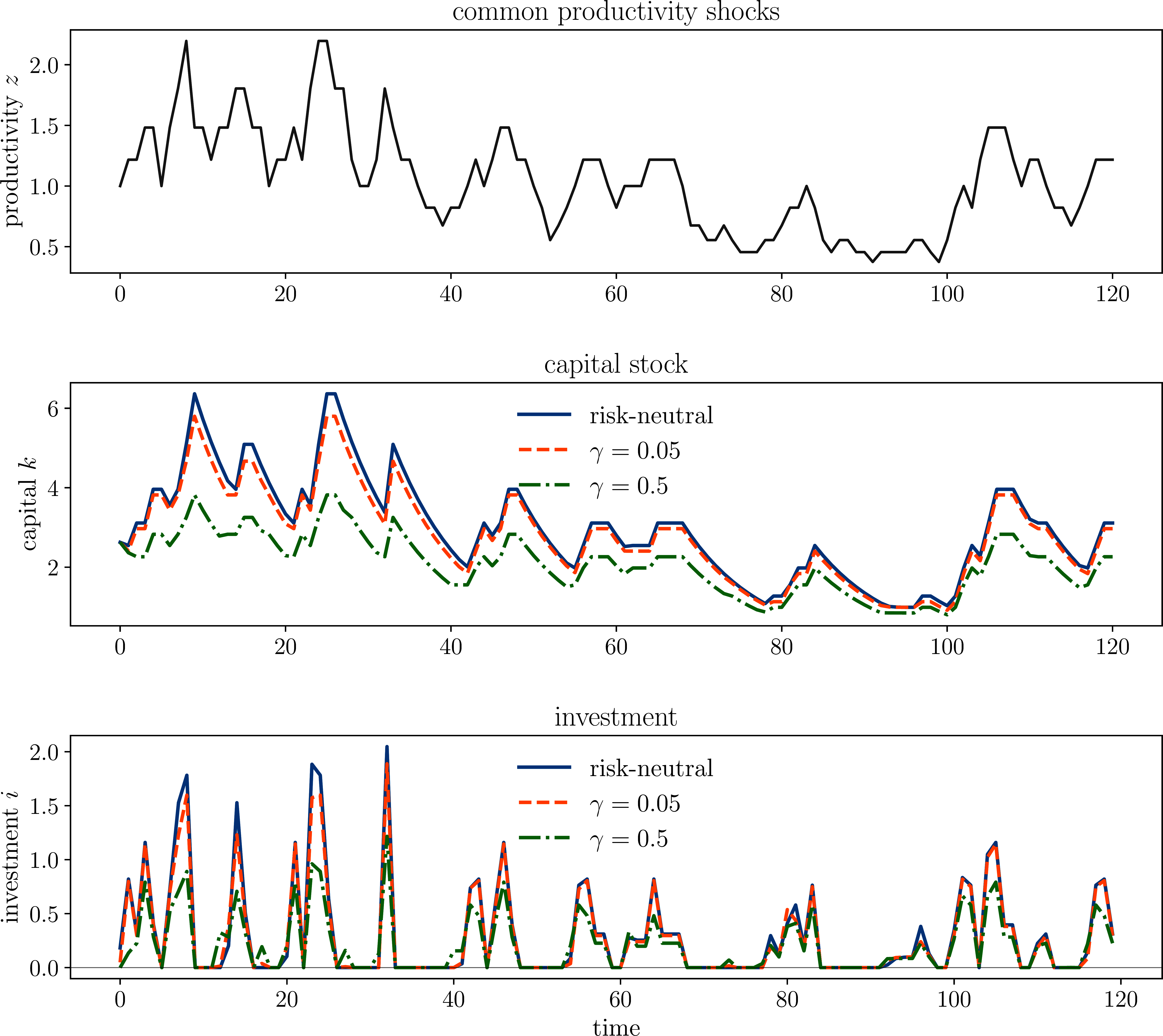
Figure 7.5 shows simulated paths for both firms facing identical productivity shocks. The risk-averse firm maintains a persistently lower capital stock and invests more cautiously throughout the sample. During periods of high productivity, the gap is especially pronounced: the risk-neutral firm boosts capital aggressively, while the risk-averse firm is restrained, anticipating the possibility of future downturns.
Figure 7.4:Investment policies: risk-neutral vs. risk-averse
Figure 7.5:Simulated paths: risk-neutral vs. risk-averse under common shocks
In Section 1.2.3.3 we discussed how concern for model misspecification can be incorporated into dynamic programs. Here we return to this topic in the context of irreversible investment. We first formulate the robust control version of the firm problem and then show how duality reduces it to the risk-sensitive case already covered by our theory.
Here k′:=i+(1−δ)k and the maximization is over i with 0⩽i⩽θf(k,z). In this case we interpret the problem as one where the manager does not fully trust the model: she fears misspecification in terms of the distribution ϕ of the shock sequence (ξt) and hence lacks full confidence when calculating expectations of continuation values. Nonetheless, she is willing to treat ϕ as a reference model. She entertains distributions ψ that deviate from ϕ, provided that they don’t assign positive probability to events that ϕ deems impossible.
The penalty term (1/γ)DKL(ψ∥ϕ) can be thought of as a soft constraint. Models further from the reference point (in terms of KL divergence) are regarded as less plausible. If γ is close to zero then the penalty term will be very large for even small deviations. Because the evaluation of the continuation value involves an infimum, only very small deviations are considered. This corresponds to greater trust in the model. Conversely, larger values of γ indicate deeper distrust.
This is a version of (7.26), with E set to the entropic certainty equivalent Eγ. Since Eγ is continuous (Exercise 7.2.6), the conditions of Proposition 7.3.2 hold under Assumption 7.3.1. As a result, for this model, the fundamental optimality properties hold, the value function v∗ lies in bcX, and VFI converges geometrically on bcX.
The above discussion shows that we do not require any new machinery to tackle the somewhat intimidating robust control version of the investment problem: a duality based approach allows us to switch to a setting where we already have all the results we need.
Figure 7.6 compares optimal investment policies under three specifications: the risk-neutral benchmark (γ→0) and the entropic certainty equivalent Eγ at two levels of ambiguity aversion.[5] As γ increases—reflecting deeper distrust in the reference model—investment falls. The manager who entertains a wider range of alternative models, and who evaluates continuation values under the worst-case distribution within the KL penalty ball, perceives a lower return to committing capital. The effect is monotone in γ: higher ambiguity aversion leads to uniformly less aggressive investment across all capital levels.
Figure 7.7 shows simulated paths for all three firms facing identical productivity shocks. The more ambiguity-averse firm maintains a persistently lower capital stock. During periods of high productivity, the differences are most visible: the risk-neutral firm ramps up capital, while the ambiguity-averse firm invests more cautiously, hedging against the possibility that the favorable conditions are less persistent than the reference model suggests.
Figure 7.6:Investment policies under ambiguity aversion
Figure 7.7:Simulated paths under common shocks with varying ambiguity aversion
We return to the setup in Section 7.2.5.1, where X, A are arbitrary metric spaces, Γ is a nonempty correspondence from X to A, and B(x,a,v)=r(x,a)+βE[v(f(x,a,ξ))]. We suppose, as in Assumption 7.2.11, that the correspondence Γ is compact-valued and continuous, the reward function r is bounded and continuous, and that the map (x,a)↦f(x,a,z) is continuous on G for all z∈Z. As discussed in Section 7.2.5.1, the fundamental optimality properties hold and VFI converges on bcX.
In Section 7.2.5.2 we extended this basic MDP analysis to settings where the aggregator has the form B(x,a,v):=r(x,a)+βEv(f(x,a,ξ)). In Proposition 7.2.10 we showed that, when E is continuous, the fundamental optimality properties hold, the value function v∗ lies in bcX, and VFI converges geometrically on bcX.
This model is called a risk-sensitive MDP. The modified expectation is an application of the entropic certainty equivalent (7.21) with θ=−γ. This modified expectation allows for parameterization of risk-sensitivity through θ, with θ<0 injecting risk-aversion. Since the entropic certainty equivalent is continuous (Exercise 7.2.6), we can apply Proposition 7.2.10. This tells us that all of the preceding convergence and optimality results apply.
Another alternative is to replace the entropic certainty equivalent with Kreps–Porteus expectations, leading to aggregator
BKP(x,a,v)=r(x,a)+β{E[v(f(x,a,ξ))ν]}1/ν(ν∈R and ν=0).
Here, in order to avoid running into trouble with exponents, we require that r>0 and take the value space V to be all functions in bX that take only positive values. We discussed such an RDP in Section 7.1.1.6.
Note, however, that the Kreps–Porteus expectation fails cash invariance, and, as such, is not a certainty equivalent (as previously discussed in Section 7.2.4.2). As a result, the preceding optimality theory does not apply. In particular, we cannot appeal to Proposition 7.2.10. Moreover, the aggregator BKP is not generally contracting, in the sense that Assumption 7.2.1 typically fails. Instead, the RDP (Γ,V,BKP) has to be treated with other methods, such as the convexity-based techniques used in Section 5.1.3.
There is, however, a multiplicative variation on the Kreps–Porteus RDP that is simple to analyze. The model is obtained by setting
BMKP(x,a,v)=r(x,a)⋅{E[v(f(x,a,ξ))ν]}β/ν,
while continuing to assume that r is everywhere positive. The parameter β is a discount factor for the multiplicative model, and is assumed to take values in [0,1). We call (Γ,V,BMKP) the multiplicative Kreps–Porteus RDP.
It turns out that the multiplicative Kreps–Porteus RDP and the additive risk-sensitive RDP (Γ,bX,BRS) are closely related—in fact they are isomorphic. To illustrate this, we take logs of the Bellman equation associated with the multiplicative Kreps–Porteus RDP, obtaining
RDPs were introduced in Chapter 8 of Sargent & Stachurski (2025) in settings where the state space is finite. The theory in this chapter extends that treatment to general state spaces. The study of contracting dynamic programs with abstract Bellman equations was begun by Denardo (1967). Extensive discussion can be found in Bertsekas (2022). (The terminology is slightly confusing: the abstract dynamic programs studied in Denardo (1967) and Bertsekas (2022) are similar to the RDPs studied in this chapter. For us, however, abstract dynamic programs are the more general objects introduced in Section 2.1.1.)
The optimality results in Section 7.2.1–Section 7.2.2 combine the RDP framework with the Blackwell contraction theory of Chapter 4. Our framework is similar to the contractive models in Bertsekas (2022). The results in Section 7.2.3 on monotonicity, concavity, uniqueness, and continuity of solutions extend related results in Bäuerle & Jaśkiewicz (2018).
In Section 7.2.2 we treated RDPs where rewards are bounded below and unbounded above. Related work can be found in Toda (2023). One approach to the reverse case—where rewards are bounded above and unbounded below—can be found in Ma et al. (2022). Their idea is to rearrange the Bellman equation so that the transformed problem has bounded rewards, allowing standard contraction mapping arguments to be applied. The transformation is inspired by the Q-function used in reinforcement learning.
Regarding Euler equations, early results along the lines of Proposition 8.3.9 were established by Mirman & Zilcha (1975) and Benveniste & Scheinkman (1979).
The certainty equivalents and risk measures discussed in Section 7.2.4 are standard tools in mathematical finance and decision theory. The dual representation theorem for convex risk measures is due to Föllmer & Schied (2002); see also Jouini et al. (2006). The quantile certainty equivalent and its risk measure counterpart (VaR) have been studied in dynamic programming environments by Castro & Galvao (2019), Castro & Galvao (2022), Almeida et al. (2024), Castro et al. (2025), and Castro & Galvao (2025), among others.
The robust control formulation in Section 7.3.3 builds on Hansen & Sargent (2001) and Hansen & Sargent (2011), who developed the multiplier preference approach to robustness in dynamic economic models. The duality between robust control and risk-sensitive preferences, which we exploit to reduce the robust problem to the entropic certainty equivalent case, is a central theme of that literature.
For a recent textbook treatment that uses the RDP framework, see Toda (2024).
If we were more cynical, we would add that existence of these two literatures also reflects the fact that researchers can publish more papers if they study the same thing under different names.
We set f(k,z)=min{zkα,y} with y=1000, α=0.3, β=0.95, δ=0.1, and θ=1.5. The exogenous state follows Zt=exp(Xt) where (Xt) is AR(1) with persistence ρ=0.9 and volatility ν=0.2, discretized via the Tauchen method. The value function is approximated on a grid via linear interpolation of v(⋅,z) for each z, and solved via VFI.
The parameterization is the same as for the risk-neutral case, with γ=0.05 and γ=0.5 for the entropic certainty equivalent. VFI converges geometrically in all cases.
Sargent, T. J., & Stachurski, J. (2025). Dynamic Programming: Finite States. Cambridge University Press.
Kristensen, D., Mogensen, P. K., Moon, J. M., & Schjerning, B. (2021). Solving dynamic discrete choice models using smoothing and sieve methods. Journal of Econometrics, 223(2), 328–360.
Rust, J. (1994). Structural estimation of Markov decision processes. Handbook of Econometrics, 4, 3081–3143.
Ma, Q., Stachurski, J., & Toda, A. A. (2022). Unbounded dynamic programming via the Q-transform. Journal of Mathematical Economics, 100, 102652.
Föllmer, H., & Schied, A. (2002). Convex Measures of Risk and Trading Constraints. Finance and Stochastics, 6(4), 429–447. 10.1007/s007800200072
Jouini, E., Schachermayer, W., & Touzi, N. (2006). Law Invariant Risk Measures Have the Fatou Property. In S. Kusuoka & A. Yamazaki (Eds.), Advances in Mathematical Economics (Vol. 9, pp. 49–71). Springer. 10.1007/4-431-34342-3_4
Denardo, E. V. (1967). Contraction Mappings in the Theory Underlying Dynamic Programming. SIAM Review, 9(2), 165–177.
Bertsekas, D. P. (2022). Abstract dynamic programming (3rd ed.). Athena Scientific.
Bäuerle, N., & Jaśkiewicz, A. (2018). Stochastic optimal growth model with risk sensitive preferences. Journal of Economic Theory, 173, 181–200.
Toda, A. A. (2023). Unbounded Markov Dynamic Programming with Weighted Supremum Norm Perov Contractions.
Mirman, L. J., & Zilcha, I. (1975). On optimal growth under uncertainty. Journal of Economic Theory, 11(3), 329–339.
Benveniste, L. M., & Scheinkman, J. A. (1979). On the differentiability of the value function in dynamic models of economics. Econometrica, 727–732.
de Castro, L., & Galvao, A. F. (2019). Dynamic quantile models of rational behavior. Econometrica, 87(6), 1893–1939.
de Castro, L., & Galvao, A. F. (2022). Static and dynamic quantile preferences. Economic Theory, 73(2–3), 747–779.
Almeida, H., Campello, M., de Castro, L. I., & Galvao Jr, A. F. (2024). A Quantile Model of Firm Investment [Techreport]. National Bureau of Economic Research.