15.1Sets
In the text we often refer to the real numbers. This set is denoted by , and we understand it to contain “all the numbers.” can be visualized as the "continuous" real line:

The term “real” sounds odd but it means "not imaginary."
is an example of a set. A set is a collection of distinct objects viewed as a whole. In the case of , the objects are numbers. Other examples of sets are the set of all rectangles in the plane, or the set of all monkeys in Japan.
If is a set, then the statement means that is contained in (alternatively, is an element of) . If is another set, then means that any element of is also an element of , and we say that is a subset of . The statement means that and contain the same elements (or, equivalently, and ). For example, if is the irrational numbers,[1] then . Also, , , , , and so on.
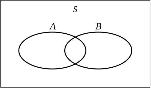
Figure 15.1:Sets and in
Commonly used subsets of include the intervals. For arbitrary and in , the open interval is defined as
while the closed interval is defined as
We also use half open intervals such as , half lines such as , and so on.
Let be a set and let and be two subsets of , as illustrated in figure 15.1.
The union of and is the set of elements of that are in or or both:
Here and elsewhere, “or” is used in the mathematical sense. It means “and/or”.
The intersection of and is the set of all elements of that are in both and :
The set is all points in that are not points in :
The complement of is the set of elements of that are not contained in :
Figure 15.2 illustrate these definitions.
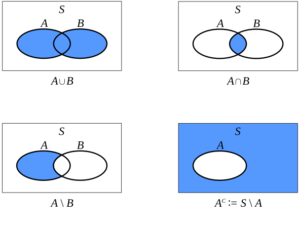
Figure 15.2:Union, intersection, and complement
For example, since consists of the irrationals and the rationals , we have
Also
The empty set is the set containing no elements. It is denoted by . If the intersection of and equals , then and are said to be disjoint.
The next fact lists some well-known rules for set-theoretic operations.
If is an infinite collection of subsets of , the union is defined as all such that for some . The intersection is all that lie in for all .
15.1.1Cartesian Products
Collections with natural order are frequently written as tuples. These are finite sequences of terms, usually denoted using notation such as or . Collections of tuples arise naturally in Cartesian products. The Cartesian product of set is the set
The vector space is one example of a Cartesian product, defined as
Thus is all tuples with for each .
A useful class of subsets of is those that are formed as Cartesian products of intervals. These are called rectangles. An example is
where are given numbers. The rectangle is shown in figure 15.3.
![Rectangle (2, 5] \times (1, 2] in \RR^2](/book-econometric-theory.mystmd/build/cart_prod-fab3b3cb675aa7b476e572c4069af3c7.svg)
Figure 15.3:Rectangle in
15.2Functions
There are two fundamental primitives in mathematics: sets and functions.[2] A function from set to set is a rule that associates to each element of a unique element of . The symbols means that is a function from to . The set is called the domain of , while is called the codomain. Figure 15.4 illustrates.
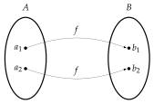
Figure 15.4:A function from to
If and then the function defined by is called the composition of and , and written as .
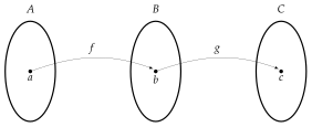
Figure 15.5:The composition
If and are points such that , then is called a preimage of . The set of preimages of can be empty, a singleton or contain multiple values. The set of points
is called the range of , and written as . Thus is in the range of if it has at least one preimage. Figure 15.6 depicts the range of a given function .
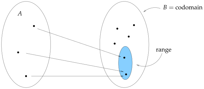
Figure 15.6:Range of
A function is called one-to-one if distinct elements of are always mapped into distinct elements of . That is, if
or, equivalently, if . Evidently is one-to-one if and only if each element of has at most one preimage under . If a function and is one-to-one, then the equation has at most one solution.
A function is called onto if ; this is if every has at least one preimage. If and is onto, then the equation has at least one solution.
Finally, is called a bijection if it is both one-to-one and onto. Bijections are sometimes called one-to-one correspondences.
If is a bijection, then the equation always has exactly one solution. We can therefore define the inverse function to , denoted by , as the map from such that is the unique with .
Part (iv) of fact 15.2.1 is illustrated in figure 15.7.
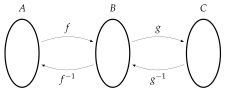
Figure 15.7:The inverse of is
15.2.1Preimage of Sets
Given any function from to and any subset of , the symbol denotes the set of points that are mapped into under . That is,
The set is called the preimage of under .
Preimages of sets interact nicely with set-theoretic operations. For example, given any , we have
,
, and
.
The equalities in (i) and (ii) also extend to infinite intersections and unions.
15.3Cardinality and Measure
For finite sets we have a fairly clear idea of what "the same size" means. For infinite sets things get tricker. It is nonetheless valuable to distinguish infinite sets according to size. To this end, when a bijection exists between sets and , they are said to have the same cardinality, and we write .
More generally, we have the following result:
This fact tells us that classifying sets by cardinality generalizes the notion of classifying sets by number of elements.
In other words, cardinality is transitive. This follows from the fact that compositions of bijections are bijections (fact 15.2.1).
A nonempty set is called finite if for some . Otherwise, is called infinite.
Sets that either are finite or have the same cardinality as are called countable.
In essence, sets formed by sequences are countable.
Uncountable sets are sets that are not countable. For example, is uncountable, as is any set that contains a nonempty open interval . Put simply, you cannot write down a sequence that will exhaust the elements of these sets. The story is similar for . (Such sets are said to have the power of the continuum.) For a beautiful proof that is uncountable, look up the diagonalization argument of Georg Cantor.
15.3.1Lebesgue Measure and Sets of Measure Zero
A set is said to have Lebesgue measure zero in if, given any , there exists a sequence of intervals such that is contained in the union of these intervals and . The definition extends to by replacing intervals with rectangles (see page for a definition of the latter).
For example, any countable set has measure zero. To see this in , let with . Fix . To each we assign an interval containing and satisfying . The union of intervals contains , and, in addition, the sum of their lengths is .
Uncountable sets can have measure zero too. For example, every linear subspace with has measure zero in . A more classical example of an uncountable set with measure zero is the Cantor set. Details can be found in many texts on analysis.
The concept of measure zero sets forms part of a branch of mathematics called measure theory. We have used aspects of measure theory in this text—for example, in our discussion of -algebras in Section 4.1.1.2 and probabilities in Section 4.1.2. The basic problem of measure theory is how to provide a well-defined notion of "measure" or "size" to sets. This is easy if we just want to assign area to a circle (area ) or rectangle, or volume to a sphere. But what about an arbitrary subset of ? Is there a well-defined and widely accepted notion of size for such a set?
The answer to this question is affirmative. The so-called Lebesgue outer measure is a map, typically denoted , that gives a natural notion of size to any set. It works by approximating arbitrary sets by simpler sets, like rectangles, and agrees with standard notions of area or volume for common geometric objects. The only problem is that it isn’t always additive, in the sense that
can fail. To get around this problem, we exclude any sets that cause (15.1) to fail. That is, we define the Lebesgue measurable sets to be those set on which additivity holds. This causes no difficulty since the discarded sets never come up in day-to-day analysis. In fact we usually focus on a smaller class of well-behaved sets, called the Borel sets. These were introduced in Section 4.1.1.2.
15.4Real-Valued Functions
For any set , if then is called a real-valued function. If and are real-valued functions, then is defined by , while is defined by . A maximizer of on is a point such that for all . The value is called the maximum of on . A minimizer of on is a point such that for all . The value is called the minimum of on .
Monotone increasing transformations of functions do not affect maximizers. To see this, let and let be monotone increasing, in the sense that if , then , and let be the function defined by . Any maximizer of on is also a maximizer of on . To see why, let . Since is a maximizer of , it must be the case that . Since is monotone increasing, this implies that . Given that was chosen arbitrarily, we have now shown that for all . In other words, is a maximizer of on .
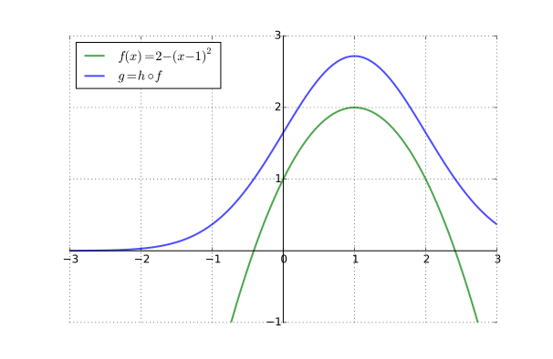
Increasing transform preserves the maximizer
15.4.1Sup and Inf
Maximizers and minimizers don’t always exist. To illustrate, consider defined by . The function has neither maximizer nor minimizer on . For example, no is a minimizer because is in and .
To negotiate this kind of problem, we can use the notion of supremum instead. If is a set, then the supremum is the unique such that (i) for every and (ii) there exists a sequence such that . For example, is the supremum of both and . The infimum is the unique such that (i) for every and (ii) there exists a sequence such that . For example, is the infimum of both and .
One can show that the supremum and infimum of any bounded set exist. The boundedness requirement can be dropped when the values and are admitted as a possible infima and suprema.
Returning to our original example with , while is not well-defined, .
The irrationals are those numbers such as and that cannot be expressed as fractions of whole numbers.
Actually functions can be represented as a special type of set containing ordered pairs, and hence in pure mathematics cannot claim to be as foundational as sets. However, for our purposes, it will be fine to think of a function as a primitive in its own right.