Probability is a technically demanding field. The main reason is that we want to assign probabilities to all manner of events. The set of possible events can be very large, and we need ways to manage this complexity. In this and the next few sections, we’ll review the basic machinery involved and why this machinery is necessary. At the same time, we’ll skip several details that would take us too far away from econometric theory. This will cost little in terms of understanding.
One concept worth mentioning before we start is countable and uncountable sets. In essence, a nonempty set S is called countable if it is either finite or can be represented as a sequence, and uncountable if is not countable. In probability theory this distinction is important. A quick review can be found in Section 15.3.
In setting up a probabilistic model, we start with the notion of a sample space, which we think of as being a "list" of all possible outcomes in a given random experiment. In general, the sample space can be any nonempty set, and is usually denoted Ω. A typical element of Ω is denoted ω. The general idea is that a realization of uncertainty will lead to the selection of a particular ω∈Ω.
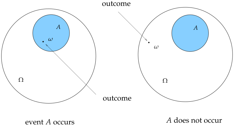
Once we have a sample space in place we can start to think about events. In the language of probability theory, an event is just a subset of Ω (with some caveats that will be addressed below). An event A occurs whenever the individual ω∈Ω selected in the random experiment happens to lie in A. Figure 4.1 illustrates.
The next thing we need to do is to assign probabilities to outcomes. One idea is to start by assigning appropriate probabilities to every ω in Ω. We could then derive the probability of events by looking at the probabilities attached to points contained in those events. It turns out, however, that this is not the best approach, at least if we want to consider uncountable Ω. Rather, the standard approach is to directly assign probabilities to subsets of Ω instead.
To see why the first approach is problematic, consider the dart throwing model in example 4.1.2, where Ω is the unit disk in R2. Imagine that hitting any point in Ω is "equally likely." We can model this by assuming that the probability the dart lands in some region A of the dartboard (some A⊂Ω) is simply proportional to the area of A.
Consider now the probability of hitting some individual point ω∈Ω. Intuitively, this should be less than the probability of hitting any region A containing ω. By choosing A to be sufficiently small in area, we can show that the probability of hitting ω is less than ϵ for any given ϵ>0. We are forced to conclude that the probability of hitting the individual point ω is zero.[1]
This example shows that in many sensible models the probability assigned to individual points in the sample space must be zero. If you reflect on this for even a moment you will agree that there is no way to build up a useful probabilistic model with such information alone. Hence we must assign probabilities directly to the events themselves.
Should we assign probabilities to every possible event—that is, to every possible subset of Ω? In the dart model above, we could say that the probability the dart lands in any region A⊂Ω is equal to the area of A divided by the area of Ω itself, which is π. In symbols,
This seems sensible enough. For example, if A=Ω, then P(A)=π/π=1, as it should be. If A is the top half of the dartboard then P(A)=0.5, and so on.
Unfortunately, if we think carefully about this approach, some cracks start to appear. What exactly do we mean by "area of A"? If A is a circle, then its area is π times the square of its radius. If A is a rectangle, then its area is the product of its two sides. But how about the area of more general subsets of Ω?
It turns out that assigning area to all subsets of Ω in a consistent way is problematic. The reason is that Ω contains an awful lot of subsets, and some of them can be manipulated to exhibit very strange phenomena. (If you are curious, look up the Banach–Tarski paradox for a hint of the problems that can occur when we try to assign notions like area or volume to arbitrary sets.) We can dream up all sorts of strange events that confound our ability to construct a sensible probabilistic model.
Because of this, when Ω is uncountable, we usually resist taking the set of events to be all subsets of Ω. Instead, we take them to be some family of "well-behaved" subsets of Ω, denoted below by F, and only assign probabilities to elements of F.
There is of course a trade-off here. If we restrict F to be a small fraction of the subsets of Ω, then assigning probabilities becomes easy and we can eliminate strange behavior. But if we make F too small, then we might not be able to assign probabilities to events that we care about. For example, in the dartboard model, if we restrict F to be the set of rectangles, then we can easily measure area and hence assign probabilities via (4.1). But this excludes interesting events such as the dart landing in the top half of the board.
How can we ensure that F is large enough? To think about this in a systematic way, suppose that A∈F, and that P(A) is well-defined and represents the “probability of event A.” Now, given that we can assign a probability to the event A, it would be unfortunate if we couldn’t assign a probability to the event “not A”, which corresponds to Ac. So normally we require that if A∈F, then Ac∈F. When this is true, we say that F is “closed under the taking of complements.”
Further, suppose that A and B are both in F, and we can assign probabilities to these events. In this case, it would be natural to think about the probability of the event “A or B”, which corresponds to A∪B. So we also require that if A and B are in F, then A∪B is likewise in F. We say that F is “closed under the taking of unions.” In fact for technical reasons it turns out that we prefer F to be closed under the taking of countable unions, which means that if A1,A2,… is a sequence of sets in F, then its union is likewise in F.
A set F of subsets of a given set Ω that satisfies all these properties is called a σ-algebra. Formally, F is a σ-algebra on Ω if
A∈F⟹Ac∈F,
A1,A2,…∈F⟹∪n=1∞An∈F, and
Ω∈F.
Note that (i) and (iii) together imply that ∅∈F. In this context, the empty set ∅ is called the impossible event. In contrast, Ω is called the certain event because it always occurs (regardless of which outcome ω is selected, ω∈Ω is true by definition).
The σ-algebra of events F we choose to pair with a given Ω can vary from problem to problem. There is however one particular σ-algebra that you should know at least something about, and that is the standard σ-algebra we use to pair with ordinary vector space RN. This σ-algebra is called the Borel sets.
To understand the idea, consider the following: The property of F being a σ-algebra seems to imply that F is a relatively rich class of sets. After all, we can take complements and unions (and intersections too—see ex. 4.4.1) without ever leaving F. However, there are trivial examples of σ-algebras, such as F:={∅,Ω}. So if we want to pin down a large and useful class of events, the best way to proceed is to assume not only that F is a σ-algebra, but also that F contains some fundamental sets that we are likely to want to attach probabilities to, such as intervals and rectangles.
In this connection, the Borel subsets of RN are defined as the smallest σ-algebra of subset of RN that contains all rectangles in RN. (See Section 15.1 if you wish to learn more about rectangles.) This definition turns out to be highly successful: Restricting attention to Borel sets does a great job of excluding the kind of strange behavior found in the Banach-Tarski paradox, and, moreover, every subset of RN we need to deal with in day to day analysis is a Borel set. These include planes and hyperplanes, circles, spheres, polygons, finite sets, and sequences of points. In what follows we use B(RN) to represent the Borel sets of RN.
Now let’s take a σ-algebra of events as given and consider how to assign probabilities to elements of F. For given event B, the symbol P(B) will be interpreted as representing "the probability that event B occurs." The way you should think about it is this:
P(B) represents the probability that when uncertainty is resolved and some ω∈Ω is selected by “nature,” the statement ω∈B is true.
In order to make sure our model of probability is well behaved, we need to put certain restrictions on P. For example, it wouldn’t do to have a B with P(B)=−93, since negative probabilities don’t make sense. The standard restrictions are imposed in the next definition:
Let Ω be a nonempty set and let F be a σ-algebra of subsets of Ω. A probabilityP on (Ω,F) is a function from F to [0,1] that satisfies
P(Ω)=1 and
P(∪n=1∞An)=∑n=1∞P(An) for any disjoint sequence of sets A1,A2,…∈F.
In this context P is also called a probability measure. Together, the triple (Ω,F,P) is called a probability space.
In the definition, axiom (i) is straightforward. We require P(Ω)=1 because, by construction, every possible ω lies in the set Ω. Axiom (ii) is called countable additivity. The concept of disjointness in the statement of the axiom is pairwise: Any distinct pair Ai,Aj share no points in common. By taking some of the sets as empty, countable additivity can be shown to imply finite additivity, which requires that
The general notion of additivity is a natural requirement for probabilistic models. It says that to find the probability of a given event, we can determine all the different (think "disjoint") ways that the event could occur, and then sum their probabilities. Probabilists boost this up to countable additivity because it helps certain limiting arguments work smoothly.
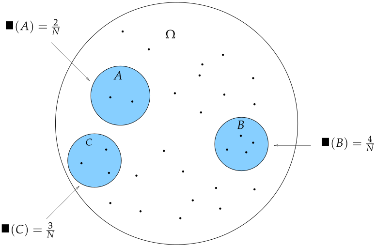
Figure 4.2 gives an illustration of additivity. Suppose that the N dots in the figure are the only possible outcomes. Suppose that each of these occurs with probability 1/N, and hence the probability of an event is the number of dots it contains divided by N. Hence P(A)=2/N, P(B)=4/N and P(C)=3/N. In addition there are 9 dots in A∪B∪C, so
P(A∪B∪C)=N9=P(A)+P(B)+P(C)
Notice how disjointness is important in making additivity work here: If the sets were not disjoint we would run the risk of double counting on the right hand side of this sum, breaking the equality.
Figure 4.2:Each of the N dots occurs with probability 1/N
The function λ from example 4.1.7 that maps Borel sets to their "area" is formally known as the Lebesgue measure. Section 15.3.1 provides a brief introduction to this concept.
Now let’s go back to the general case, where (Ω,F,P) is an arbitrary probability space. From the axioms, we can derive a surprising number of properties. Let’s list the key ones, starting with the next fact.
(Here Ac=Ω∖A. See Section 15.1 for a review of set-theoretic operations.)
To prove fact 4.1.1, note that when A⊂B, we have B=(B∖A)∪A. Since B∖A and A are disjoint, additivity of P now gives
P(B)=P(B∖A)+P(A)(whenever A⊂B)
This equality implies (i)–(iv) of fact 4.1.1. Rearranging gives (i), while nonnegativity of P gives (ii). Specializing to B=Ω gives (iii), and setting B=A gives (iv).
The property A⊂B⟹P(A)⩽P(B) is called monotonicity, and is both fundamental and intuitive: If A⊂B, then we know that B occurs whenever A occurs, since ω lands in B whenever it lands in A. Hence the probability of B should be no smaller. Many results in probability turn on this idea.
Exercise 4.4.2 asks you to prove this. It follows from fact 4.1.2 that for any A,B∈F, we have P(A∪B)⩽P(A)+P(B). This inequality is called subadditivity. Thus probabilities are subadditive over arbitrary pairs of events and additive over disjoint pairs.
It represents the probability that A will occur, given the information that B has occurred. For the definition to make sense, we need P(B)>0. Events A and B are called independent if P(A∩B)=P(A)P(B). More generally, events A1,…,AN∈F are called independent if
Note that if A and B are independent, then the conditional probability of A given B is just the probability of A.
To state the next result, we need the concept of a partition of Ω, by which we mean a countable set of events {Bm}m⩾1 with the property that distinct pairs are disjoint and ∪m⩾1Bm=Ω.
The following fact is known as the law of total probability.
The proof is as follows: It is a basic result from set theory that A∩(∪mBm)=∪m(A∩Bm). From this equality, the definition of a partition and countable additivity of P, we get
In some probability courses, a random variable is defined as a “value that changes randomly,” or something to that effect. This is a fairly useless definition. A better definition of a random variable is a function x from a sample space Ω into R. Think of it this way:
“Nature” picks out an element ω in Ω according to some probability.
The random variable x sends this ω into numerical value x(ω).
Thus a random variable is a map x that converts outcomes in sample space—which can be any kind of object—into numerical outcomes. This is valuable because numerical outcomes are easy to order, add, subtract and so forth. In other words, random variables "report" the outcome of an experiment in a format amenable to further analysis.
The random variable y in (4.7) is an example of a binary (or Bernoulli) random variable, which is a random variable taking values in the set {0,1}. There is a generic way to create binary random variables that often comes in handy, using indicator functions. If Q is a statement, such as “on the planet Uranus, there exists a tribe of three-headed monkeys,” then 11{Q} is considered as equal to 1 when the statement Q is true, and zero when the statement Q is false. Another common variation on the notation is, for arbitrary A∈F,
11A(ω):=11{ω∈A}:={10if ω∈Aotherwise
So defined, 11A is a binary random variable. In fact any binary random variable x can be expressed as 11A by setting A:={ω∈Ω:x(ω)=1}.
Here equality means when evaluated at any ω∈Ω. See exercise 4.4.5.
Given random variable x, you will often see notation such as
{x has some property}
This is a shorthand for the event
{ω∈Ω:x(ω) has some property}
Another notational convention you should be aware of is that, for random variables, equalities, inequalities and arithmetic operations should be interpreted pointwise. For example,
We’ve omitted a technical detail in our construction of random variables. It arises because we cannot always take the set of events F to be the set of all subsets of Ω (since assigning probabilities to arbitrarily complex sets causes problems—see the discussion in Section 4.1.1).
To explain, let (Ω,F,P) be any probability space. Let B be any subset of R and consider evaluating the probability
P{x∈B}:=P{ω∈Ω:x(ω)∈B}
Here x is some function from Ω to R. Now observe that if we put no restrictions on x, we might end up in a mess. The reason is that we have no way of being sure that the set {ω∈Ω:x(ω)∈B} is in fact an element of F. Since P is only defined over elements of F (i.e., for bona fide events), it is possible that P{x∈B} is undefined.
To prevent such embarrassment, it’s standard to put some restrictions both on x and B that ensure {x∈B}∈F. For B, we naturally restrict attention to B(R), the Borel subsets of R, since we know these sets to be both relatively well behaved and common enough to satisfy our purposes (see Section 4.1.1). For x, we simply require that {x∈B}∈F whenever B is a Borel set. Thus, our formal definition is that a random variable on (Ω,F) is a function x:Ω→R satisfying
These kinds of functions are also sometimes called F-measurable functions. In other texts you will see (4.9) expressed using preimage notation. In the preimage notation, x−1(B) is all ω∈Ω such that x(ω)∈B. This is just the left-hand side of (4.9), so we can rewrite (4.9) as
So far so good. If x is a random variable, then {x∈B} is a well-defined event for every B∈B(R). But suppose now that we want to discuss some transformation of x. For example, we might be interested in the properties of y:=ex. Is y also a random variable? That is, is {y∈B} always a well-defined event?
The answer to this question is affirmative provided that our transformation satisfies a regularity condition called Borel measurability. Formally, f:R→R is called Borel measurable, or B-measurable, if
Thus f "pulls back" Borel sets to Borel sets. Although we omit the details, the class of B-measurable functions is vast (any continuous function, any increasing function, etc., etc.), and all transformations we work with below are B-measurable.
So why is B-measurability of f the key to ensuring that y=f(x) is a random variable? Suppose that f is B-measurable and that x is a random variable. We claim that {y∈B}∈F for all B∈B(R). This holds because
Our next task is to define expectations of random variables and state their basic properties. Elementary probability courses define expectations by summing or integrating functions over densities. The view of a random variable as a function on a sample space plays no part in these definitions. However, when we move to more sophisticated arguments, particularly those involving a large number of random variables, we need a better definition. This section outlines the modern treatment of expectations found in probability and statistics. As we’ll see later, the definition in this section is a generalization of the elementary definition. The two agree whenever the latter is well defined.
For finite random variables (i.e., random variables with finite range) the expectation is just the sum of all possible values of the variable, weighted by the corresponding probabilities. More formally, given probability space (Ω,F,P) and random variable x taking only finitely many distinct values s1,…,sJ, the expectation of x is defined as
4.1.4.1Expectations for Arbitrary Random Variables¶
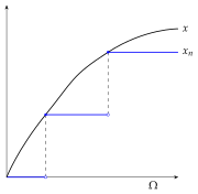
Definition (4.12) only applies for random variables with finite range. We still need to define expectation for general x. This is done by bootstrapping up from the finite case. The procedure is based on approximating arbitrary random variables with finite random variables. One finite approximation xn to an arbitrary random variable x is shown in figure 4.3. The approximation can be improved without limit if we allow xn to take a larger and larger number of distinct values. This process yields a sequence of finite random variables xn converging to x (e.g., see Çinlar (2011), lemma 2.16). The expectation of x is then defined as
The value Ex is also referred to as the Lebesgue integral of x with respect to P, with the alternative notation Ex=∫x(ω)P(dω).
Figure 4.3:Finite approximation to a general random variable
Can we be sure that the limit in (4.14) makes sense? Suppose first that x is nonnegative (i.e., x(ω)⩾0 for all ω∈Ω). It can be shown that the sequence {xn} approximating x can then be chosen so that Exn is monotone increasing and hence convergent, and that the limiting value does not depend on the particular approximating sequence {xn}. See, for example, Dudley (2002), proposition 4.1.5. Hence Ex is well defined, although we cannot rule out divergence of the sequence, which gives Ex=∞.
We’ve assumed that x is nonnegative. If we drop this assumption, we can still treat x with similar methods by writing it as the difference between two nonnegative random variables. Typically this is done by writing x=x+−x−, where x+:=max{x,0} and x−:=−min{x,0}. Both x+ and x− are nonnegative random variables. The expectation can then be defined as
This is fine except that (4.15) might have the form ∞−∞, which isn’t well-defined. For this reason we often restrict attention to integrable random variables, which are all random variables x such that E∣x∣<∞. Since x+⩽∣x∣ and x−⩽∣x∣, this is enough to ensure that (4.15) is well-defined.
The definition of E given in this section doesn’t really tell us how to calculate Ex in specific instances, but we’ll see how to do so in Section 4.2.5.
Let’s summarize the main results concerning expectations and list some properties of this operation.
Since we only know how to take expectations of random variables, the expression Eα in part (i) should be understood as the expectation of a constant random variable everywhere equal to α. (We could write this object more precisely as α11Ω.) That the expectation equals α was already established in example 4.1.15. It also follows from (ii) and (iv), by taking x=11Ω and β=0.
Part (ii) follows from example 4.1.16. It is restated here to emphasize this fundamental link between probabilities and expectations. Part (iii) is called monotonicity of expectations. The statement x⩽y means that x(ω)⩽y(ω) for all ω∈Ω. Exercise 4.4.23 asks you to prove this monotonicity in a special case. For a general proof see lemma 4.1.9 of Dudley (2002). Part (iv) is called linearity of expectations. Here αx+βy should be understood as the random variable (αx+βy)(ω):=αx(ω)+βy(ω). Exercise 4.4.13 and Exercise 4.4.14 ask you to check linearity in some special cases. For the general case see theorem 4.1.10 of Dudley (2002).
As an exercise, let’s use these results to prove that if x is a finite random variable with range {sj}j=1J and h is any B-measurable function, then h(x) has expectation
Let x be a random variable and let k∈N. If xk is integrable, then
E[xk] is called the kth moment of x.
E[(x−Ex)k] is called the kth central moment of x.
If E[∣x∣k]=∞, then the kth moment is said not to exist. For some random variables even the first moment does not exist. For others every moment exists.
Exercise 4.4.24 asks you to confirm this. The next fact is called the Cauchy–Schwarz inequality for random variables. Its proof will be given later, once we’ve covered orthogonal projection (ex. 5.4.15).
The second central moment of x is called the variance of x:
varx:=E[(x−Ex)2]
This gives a measure of the dispersion of x. The standard deviation of x is
σx:=varx
The covariance of random variables x and y is defined as
cov[x,y]:=E[(x−Ex)(y−Ey)]
Part (i) follows from (ii)–(iii), the Cauchy–Schwarz inequality and fact 4.1.7. Parts (ii)–(iii) follow from linearity of E and some simple manipulations.
Some simple implications of this fact are that
var[α+βx]=β2var[x] and
var[αx+βy]=α2var[x]+β2var[y]+2αβcov[x,y].
The correlation of x and y is defined as
corr[x,y]:=σxσycov[x,y]
If corr[x,y]=0, we say that x and y are uncorrelated. Positive correlation means that corr[x,y] is positive and negative correlation means that corr[x,y] is negative. The first part of the next fact follows immediately from fact 4.1.8; the second is just algebra.
As an application of covariance and a prelude to our discussion of prediction, let’s consider the problem of predicting the value of a random variable y given knowledge of the value of a second random variable x (and also knowledge of the underlying probability distributions, which makes this a problem in probability rather than statistics). Thus we seek a function f such that f(x) is close to y on average. To measure the latter, we will use mean squared error, which amounts in this case to
E[(y−f(x))2]
As we’ll see in Section 5.2.5, the minimizer of the mean squared deviation over all functions of x is obtained by choosing f(x)=E[y∣x], where the right-hand side is the conditional expectation of y given x. Here we’ll consider the simpler problem of finding a good predictor of y within the class of “linear” functions
Hℓ:={ all functions of the form ℓ(x)=α+βx}
(We defer to common usage and call such functions linear in this context, despite the fact that they are, in general, affine; see example 2.1.23.) Thus we consider the problem
If you’ve studied simple linear least squares regression before, you might realize that α∗ and β∗ are the “population” counterparts of coefficient estimates in an empirical setting. In example 4.1.18, this allows us to take the coefficient β∗ as the definition of an asset’s beta, independent of any particular data set. If we wish to evaluate β∗, however, we need to use data, since the underlying probabilities, and hence the expectation operator E, are not observable. It is at this stage that the population regression is replaced by simple linear least squares using data. More on this below.
Any random variable x on a given probability space (Ω,F,P) assigns to each Borel set B⊂R a number P{x∈B} indicating the probability that x lies in B. While this is an important construction, as a means of specifying probabilities for outcomes in R, it is somewhat indirect. When building statistical models, it’s often more convenient to assign probabilities to subsets of R directly. This is typically done by specifying a distribution over R. In this section we look at how one might go about specifying such distributions.
How can we specify probabilities over subsets of R? In Section 4.1.1.2–Section 4.1.2 we learned how to construct a set of events F on an arbitrary sample space Ω and define a probability measure P on F. If we want to describe probabilities over R, then the natural thing to do is to repeat the process with Ω specialized to R. For the set of events over R we take the Borel sets B(R), as discussed in Section 4.1.1.2. A probability measure defined over B(R) is called a law or distribution.
Distributions will be represented by symbols such as P and Q. Referring back to the definition, a distribution P is a map from B(R) to [0,1] such that
P(R)=1 and
P(∪n=1∞Bn)=∑n=1∞P(Bn) for any disjoint sequence {Bn}.
Being a probability measure, P satisfies all the properties in fact 4.1.1. If there exists a Borel set S with P(S)=1, then we say that P is supported on S.
Probability measures are both general and comprehensive. Each one pins down probabilistic information for every event in R that we might care about in econometrics or statistics. At the same time, this kind of generality can also be a hindrance. For example, it’s not a trivial task to assign a specific value P(B) to every single Borel set.
Fortunately, we can characterize distributions more succinctly. To begin, we recall the notion of a cumulative distributed function, or CDF, which is any function F:R→[0,1] satisfying
monotonicity: s⩽s′ implies F(s)⩽F(s′),
right-continuity: F(sn)↓F(s) whenever sn↓s, and
lims→−∞F(s)=0 and lims→∞F(s)=1.
CDFs and distributions on R can be put in one-to-one correspondence as follows: First, it’s true by definition that any two distributions Q and P satisfying Q(B)=P(B) for all B∈B(R) are the same distribution, but it’s also true that if Q(B)=P(B) for all sets B of the form (−∞,s], then Q and P are again the same distribution. In other words, a distribution P is entirely characterized by the values of the function
Moreover this function turns out to have properties (i)–(iii) above. The next fact summarizes the relationship between F and P.
For a full proof, see Williams (1991), lemma 1.6, or Dudley (2002), theorem 9.1.1. Here let’s restrict ourselves to showing that the function F in (4.24) satisfies part (i) of the definition of a CDF. To see why (i) holds for this F, observe that s⩽s′ implies (−∞,s]⊂(−∞,s′]. Part (ii) of fact 4.1.1 then gives P((−∞,s])⩽P((−∞,s′]). Hence F(s)⩽F(s′) as claimed.
CDFs are relatively easy to specify and work with. Here are some examples.
There are two important sub-cases for distributions: the discrete case and the absolutely continuous case. As we’ll see, in these two sub-cases distributions have nice visual representations and expectations are easy to compute. Almost all "named" distributions fall into one of these two categories.
A distribution P is called discrete if it is supported on a countable set; that is, if there exists a countable set {sj}j⩾1 with P({sj}j⩾1)=1. For such a P let
pj:=P{sj}:=P({sj})=probability mass on the single point sj
Property (ii) of P and P({sj}j⩾1)=1 imply that ∑j⩾1pj=1 (ex. 4.4.15). Hence {pj}j⩾1 is an example of a probability mass function, or PMF, which is any nonnegative sequence (finite or infinite) that sums to unity.
Together, {sj}j⩾1 and {pj}j⩾1 characterize the underlying distribution. For example, we can express the CDF corresponding to P via (4.24) as
This is intuitive: F(s) represents the probability of an outcome in (−∞,s] under P. Since P puts all its probability mass on {sj}j⩾1, this should equal the sum of the probabilities of hitting sj over all sj⩽s.
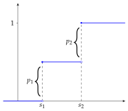
Figure 4.7 gives a visualization when {sj}j⩾1={s1,s2}. F is a step function, with a jump up of size pj at point sj. The CDF is right-continuous but not continuous.
Another case of interest is what elementary books on probability call the "continuous" case, where distributions can be described by densities. A density is a nonnegative function p on R that integrates to 1. We say that distribution P is represented by density p (or has density p) if p is a density and
Recall from our discussion in Section 4.2.1 that distributions are characterized by their values on simple sets, like half lines of the form (−∞,s]. Thus, if p is a density and
Not every distribution has a density representation. An exact necessary and sufficient condition for existence is absolute continuity. A distribution P on the Borel subsets of R is called absolutely continuous if P(B)=0 whenever B has Lebesgue measure zero. A definition of the latter property is given in Section 15.3.1, although for us it is enough to know that any countable subset of R has Lebesgue measure zero. This leads to the following fact:
Compare with the discrete distributions, which put all mass on a countable set. One important implication of fact 4.2.2 is that individual points receive no probability mass under absolute continuity, and the corresponding CDF contains no jumps. In fact, when (4.27) holds, the fundamental theorem of calculus tells us that F(s)=P((−∞,s]) is differentiable at all continuity points of p, and, in particular,
F′(s)=p(s)for all s∈R such that p is continuous at s
We all understand what it means to take the ordinary integral ∫abh(s)ds of a well-behaved function h on some interval [a,b]. Sometimes we want to weight this integral, assigning more mass to different regions of [a,b]. This leads to integrals such as ∫abh(s)p(s)ds. For example, h could be a welfare function and p might record the density of agents of a certain type. In a probabilistic context, p might be a density indicating probabilities of outcomes, h might be a payoff function and ∫abh(s)p(s)ds would be expected payoff.
We now wish to give meaning to expressions of the form ∫h(s)P(ds) that can be viewed as generalizations of these integrals. The nature of the generalization is that the probability P might not have a density, and yet we still want to compute a weighted integral using P. As motivation we’ll continue with the previous example, where h(s) is the payoff from outcome s∈R, and the likelihood of outcomes is determined by probability measure P. To provide some basic regularity, we assume that h is a B-measurable function on R.
Actually our task is straightforward given the foundations already laid. In particular, we already have a general notion of integration suitable for understanding the expression ∫h(s)P(ds). In Section 4.1.4 we saw how to take an arbitrary probability space (Ω,F,P) and construct an expectation operator E that assigns to any integrable random variable a notion of expectation. Expectations can be thought of as integrals, as suggested by the alternative notation ∫x(ω)P(dω) for Ex used in (4.16).
So now take our distribution P on R and consider (R,B(R),P) as a probability space. This new probability space has its own expectation operator EP. (See fact 4.1.5 if you wish to refresh your memory on this point.) Moreover we can use it to take the expectation of the payoff function h, which, being a B-measurable function on R, is by definition a random variable on (R,B(R),P). This gives us a value EPh, which is exactly the integral we’re after:
EPh:=:∫h(s)P(ds):=the expectation of h under P
While the preceding discussion gives a neat definition of ∫h(s)P(ds), it would be disappointing if this definition didn’t lead us back to familiar expressions like ∫h(s)p(s)ds when P has a density. Fortunately, it does:
For a proof of fact 4.2.3, see §6.12 of Williams (1991).
In Section 4.1.3 we defined random variables. Over the last few sections we’ve defined and discussed distributions over the Borel subsets of R. Our next job is to connect them. We’ll see that the connection runs in both directions: Every random variable defines a distribution on R. Conversely, given any distribution, we can reverse engineer a random variable having that distribution.
To begin, let x be a random variable on some probability space (Ω,F,P). By construction, the probability P{x∈B} is well-defined for every B∈B(R) (see (4.9)). The values obtained from this expression when x is held fixed and B is varied is called the distribution of x. In particular, the set function P defined by
is both the distribution of x and also a distribution in the sense of Section 4.1.3 (i.e., a probability measure over the Borel sets). It records the probabilities of all outcomes of interest for the variable x when regarded as a single entity.[3] In what follows we write L(x) for the distribution (or "law") of x. The relationship in (4.30) is summarized by writing L(x)=P.
By (4.24), the CDF corresponding to the distribution P of x satisfies
Sometimes F is called the distribution function or just distribution of x. Since F characterizes P, we also write L(x)=F to indicate that F represents the distribution of x.
Indeed, if a⩽b, then {a<x⩽b}={x⩽b}∖{x⩽a} and {x⩽a}⊂{x⩽b}. Applying fact 4.1.1 gives
P{a<x⩽b}=P{x⩽b}−P{x⩽a}=F(b)−F(a)
From (4.31) we get for each random variable a uniquely defined CDF. It’s also true that for every CDF F, there exists a probability space (Ω,F,P) and a random variable x:Ω→R such that L(x)=F; Section 7.4.1 outlines one construction.
In what follows, if L(x)=P and P has density p, we’ll say that x has density p. If the distribution of x is discrete, we’ll call x a discrete random variable. In the former case, where the distribution of x is absolutely continuous, no probability mass is placed on finite sets, leading to the next fact.
One often needs to obtain the distribution of the transform of a random variable. This is easy in the monotone case.
To see why, observe that under these hypotheses ψ−1 exists and is (weakly) increasing. Hence
P{y⩽s}=P{ψ(x)⩽s}=P{x⩽ψ−1(s)}=F(ψ−1(s))
Note how monotonicity is used in the second equality. (A related result can be derived for the strictly decreasing case, where the direction of the inequality flips.)
An important related question is to determine when y=ψ(x) has a density, and what the form of this density is.
Exercise 5.4.1 asks you to confirm (4.32). The term diffeomorphism just means that ψ is a bijection on R and both ψ and its inverse are differentiable.
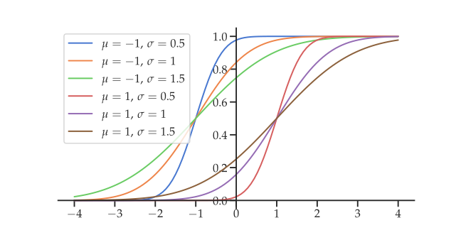
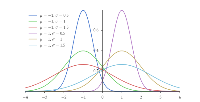
When x is standard normal, this implies that y=μ+σx is N(μ,σ2), as can be seen by taking p to be the standard normal density ϕ and comparing with the expression for the N(μ,σ2) density.
Fact 4.2.7 can be generalized. See, for example, theorem 15.5 of Schilling (2005).
Let x be a random variable on probability space (Ω,F,P). The distribution of x encodes all the information necessary to calculate expectations of x or of any B-measurable transformation h(x). This is clearest when x is finite. For example, suppose that L(x)=P, that h:R→R is any B-measurable function, and that P puts all mass on finite set {sj}j=1J. Let {pj} be the PMF of P, so that pj=P{sj}. Applying the definition of expectations (see in particular (4.17)) and using P{x=sj}=P{sj} gives
Comparing this with (4.28), we can also write Eh(x)=∫h(s)P(ds). Put differently, the expectation of h(x) on (Ω,F,P) is equal to the expectation of h on (R,B(R),P). This is also true in the infinite case (see, e.g., theorem 5.2 of Çinlar (2011)), as stated in the next fact.
In Section 4.1.5 we defined moments of random variables. For example, Exk is the kth moment of x, assuming it exists. It is clear from fact 4.2.8 that any two random variables with the same distribution share the same moments. Hence moments are best thought of as a property of the distribution, not the random variable. Thus we define
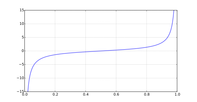
In this section it will be convenient to describe distributions in terms of CDFs. So let F be a CDF on R, which, for the moment, we assume to be strictly increasing. Given τ∈(0,1), the τth quantile of F is the ξ∈R that solves F(ξ)=τ. Under our assumptions on F, such a ξ exists and is uniquely defined. The 0.5th quantile is called the median of F. It provides a measure of central tendency for the distribution.
We can of course express the τth quantile of F using the inverse function:
If F is not strictly increasing, then there exist at least two distinct points s,s′ such that F(s)=F(s′), and hence F−1 in (4.34) is not well-defined. This problem is negotiated by setting
(See Section 15.4.1 for a definition of inf.) In the case where F is strictly increasing, (4.35) reduces to (4.34).
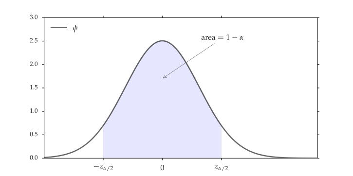
The quantile function is used in hypothesis testing to determine critical values. Let’s outline a common scenario.
Here symmetry of p means that p(s)=p(−s) for all s∈R. This is equivalent to F(s)=1−F(−s), as can be seen by differentiating or integrating. Exercise 4.4.18 asks you to prove fact 4.2.9.
Now take a random variable x with L(x)=F and constant α∈(0,1) as given, and consider the c that solves P{−c⩽x⩽c}=1−α.
To see this, fix α∈(0,1) and let c be as in (4.36). From fact 4.2.9, we have
P{∣x∣⩽c}=2F(c)−1=2F[F−1(1−α/2)]−1=1−α
In the case where F is the standard normal CDF Φ, this value c is usually denoted by zα/2. We will adopt the same notation:
The modern axiomatic treatment of probability based on measure theory was formulated in the 1930s by Andrei N. Kolmogorov. A discussion of his life and work can be found in Kendall et al. (1990). Nice introductory texts on measure-theoretic probability include Williams (1991) and Rosenthal (2006). Beautiful expositions at a slightly higher level can be found in Dudley (2002), Çinlar (2011), and Pollard (2002).
Is this true? If ω=ω0 is an infinite sequence containing only zeros, then {n∈N:bn=1}=∅. What is x(ω0) in this case? The convention is min∅=∞, which is reasonable, but now x can take the value ∞. However, in most applications this event has probability zero. We could set x(ω0)=0 without changing anything significant. Now we’re back to a well-defined function from Ω to R.
Çinlar, E. (2011). Probability and Stochastics. New York: Springer.
Dudley, R. M. (2002). Real Analysis and Probability (2nd ed.). Cambridge, UK: Cambridge University Press.
Williams, D. (1991). Probability with Martingales. Cambridge, UK: Cambridge University Press.
Schilling, R. L. (2005). Measures, Integrals and Martingales. Cambridge, UK: Cambridge University Press.
Kendall, D., Batchelor, G., Bingham, N., Hayman, W., Hyland, J., Lorentz, G., Moffatt, H., Parry, W., Razborov, A., & Robinson, C. (1990). Andrei Nikolaevich Kolmogorov (1903–1987). Bulletin of the London Mathematical Society, 22(1), 31–100.
Rosenthal, J. S. (2006). A first Look at Rigorous Probability Theory (2nd ed.). New Jersey: World Scientific.
Pollard, D. (2002). A User’s Guide to Measure Theoretic Probability (Vol. 8). Cambridge, UK: Cambridge University Press.