5 Modeling Dependence

To study relationships between random variables we need to add more concepts to our toolkit. In this chapter we review multivariate distributions and give a rigorous construction of conditional expectation.

5.1Random Vectors and Matrices¶

Let’s begin with random vectors and matrices.

5.1.1Random Vectors¶

In Section 4.1.3 we defined a random variable to be a function $x \colon \Omega \to \RR$ with the property that $\{x \in B\}$ is an event for any Borel set $B \in \bB(\RR)$. The definition of a random vector is analogous. A random vector $\boldx$ in $\RR^N$ is a function from $\Omega$ to $\RR^N$ with the property that

This is just (4.9) with $\bB(\RR^N)$ replacing $\bB(\RR)$. In statistical applications we can almost always cook up a sample space $\Omega$ and a set of events $\fF$ on $\Omega$ such that all random vectors we care about satisfy (5.1).^[1]

It’s also possible to define a random vector $\boldx$ in $\RR^N$ as a tuple of $N$ random variables $(x_1, \ldots, x_N)$. The two definitions are equivalent. As with ordinary vectors, random vectors have no intrinsic shape, and we’ll write them in rows or columns according to convenience. However, in expressions involving matrix multiplication, random vectors will default to column vectors unless otherwise stated.

The definition of a random vector ensures that $\{\boldx \in B\}$ is a well-defined event for every $B \in \bB(\RR^N)$. If we want to ensure that some transformation $\boldy = f(\boldx)$ is likewise a random vector, we need a restriction on $f$ so that $\{\boldy \in B\}$ is also a well-defined event. The appropriate restriction is $\bB$-measurability, which, analogous to the scalar case , means that $f \colon \RR^N \to \RR^M$ satisfies $f^{-1}(B) \in \bB(\RR^N)$ for all $B \in \bB(\RR^M)$. As in the scalar case, every kind of transformation we use in this text is $\bB$-measurable, so the restriction is never binding.

Expectations of random vectors are defined element-by-element. In particular, if $\boldx = (x_1, \ldots, x_N)$ is a random vector in $\RR^N$, then its expectation $\EE \boldx$ is defined as the vector of expectations

An $M \times N$ random matrix $\boldX$ is an $M \times N$ array of random variables. Its expectation is defined as

Fact 5.1.1 is obtained by repeated application of the linearity of scalar expectations stated in fact 4.1.5.

The variance–covariance matrix of a random vector $\boldx$ in $\RR^N$ with $\boldmu := \EE \boldx$ is the $N \times N$ matrix

Expanding this out gives

The $j,k$th term is the scalar covariance between $x_j$ and $x_k$ and the principal diagonal contains the variance of each $x_n$.

The cross-covariance between random vectors $\boldx$ and $\boldy$ is defined as

Evidently $\var[\boldx] = \cov[\boldx, \boldx]$.

Here’s a useful fact concerning expectations of quadratic forms. The proof is a solved exercise (see ex. 5.4.7).

5.1.2Multivariate Distributions¶

The definition of a distribution over $\RR^N$ generalizes that of a distribution over $\RR$ given in Section 4.2.1. In particular, a distribution or law $P$ on $\RR^N$ is a probability measure over the Borel sets $\bB(\RR^N)$. By definition, it satisfies $P(\RR^N) = 1$ and $P(\cup_{n=1}^{\infty} B_n) = \sum_{n=1}^\infty P(B_n)$ for any disjoint sequence $\{B_n\}$ in $\bB(\RR^N)$. See also the properties of probability measures listed in fact 4.1.1.

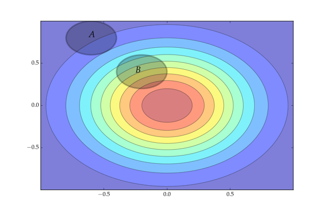
Figure 5.1 shows a visualization of a distribution $P$ on $\RR^2$, with hot colors indicating regions of high probability. (The distribution is multivariate Gaussian, to be defined below.) The sets $A$ and $B$ are typical Borel sets. In the figure, $B$ has the same area as $A$ but is assigned greater probability by $P$. By additivity, we know that $P(A \cup B) = P(A) + P(B)$ must hold.

As was the case for $\RR$, distributions on $\RR^N$ are fully characterized by their values on certain more elementary families of subsets of $\RR^N$. For example, for any two distributions $Q, P$ on $\RR^N$,

where $\rR$ denotes the family of all cylinder sets

or, specializing further, the family of all rectangles^[2]

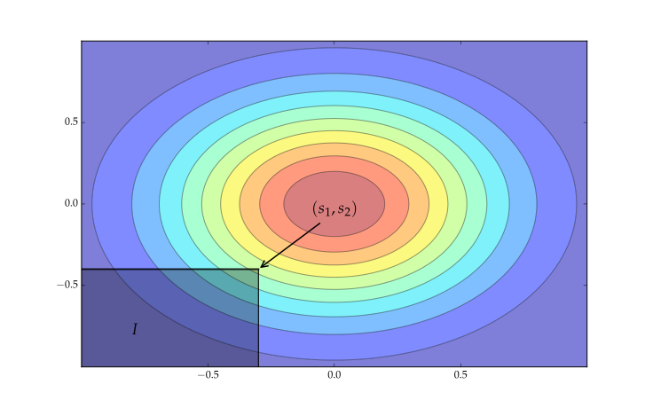
(See prop 3.7 of Çinlar (2011).) Figure 5.2 shows an example set $I = (-\infty, s_1] \times (-\infty, s_2]$ in the case of $\RR^2$.

Thus, analogous to (4.24), any distribution $P$ on $\RR^N$ is characterized by the function

This is an example of a multivariate cumulative distribution function, which is a function $F \colon \RR^N \to [0, 1]$ that is

As in the one-dimensional case, we will call a distribution $P$ on $\RR^N$ discrete if $P$ is supported on a countable subset of $\RR^N$, and absolutely continuous if $P(B) = 0$ whenever $B$ has zero Lebesgue measure. The latter condition is again necessary and sufficient for existence of a density representation, by which we mean existence of a density $p$ on $\RR^N$ such that

The right-hand side of (5.4) is a multivariate integral that we can write out more explicitly as

Conversely, if $p$ is any density on $\RR^N$, then (5.4) defines a distribution.

Let’s describe one important way to construct multivariate distributions.

This distribution is called the product distribution of $P_1, \ldots, P_N$. If $P_n = P$ for all $n$, then we’ll call $\mathring P$ the $N$th product of $P$. The uniqueness part of fact 5.1.4 follows from the claim above that distributions on $\RR^N$ are uniquely pinned down by their values on cylinder subsets of $\RR^N$. As we’ll see, product distributions correspond to joint distributions of independent random variables.

5.1.2.1Marginals of Multivariate Distributions¶

Given any distribution $P$ on $\RR^N$, the $n$th marginal distribution of $P$ is the distribution on $\RR$ defined by

Here $B$ is the $n$th element of the Cartesian product. We can also write this as

The $n$th marginal tells us the probabilistic implications of $P$ when we only concern ourselves with the outcomes for the $n$th coordinate. From $P_n$ we can also extract the marginal CDF $F_n$ via (4.24).

If $P_n$ is absolutely continuous, it has density $p_n$. When the joint distribution $P$ has a density $p$, the marginal distribution $P_n$ has a density, and $p_n$ can be obtained directly from $p$ by integrating out the other variables. For example, in the bivariate case,

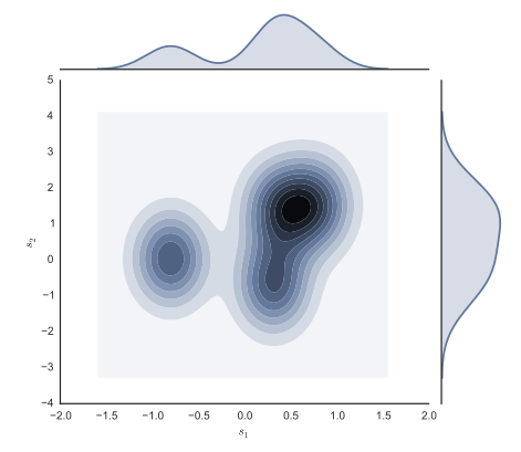
Figure 5.4 shows a bivariate density represented by contours and the two marginals obtained from projecting onto each axis.

In general, the joint distribution cannot be determined from the marginals alone, since the marginals do not tell us about the interactions across coordinates. The exception is when there is no interaction. This is the case for product distributions, as described in fact 5.1.4 and further discussed in Section 5.1.4.

5.1.3Distributions of Random Vectors¶

Let $\boldx$ be a random vector in $\RR^N$. The distribution of $\boldx$ is the probability measure $P$ on $\bB(\RR^N)$ defined by

In this context, $P$ is also called the joint distribution of $x_1,\ldots, x_N$, and we write $\lL(\boldx) = P$. The joint distribution can also be represented by the multivariate CDF $F \colon \RR^N \to [0, 1]$ defined by (5.3), which in this case can be written as $F(s_1,\ldots,s_N) = \PP\{ x_1 \leq s_1, \ldots, x_N \leq s_N\}$, or, in vector notation,

It follows from (5.4) that when the distribution $P$ of $\boldx$ is absolutely continuous, there exists a nonnegative function $p$ on $\RR^N$ satisfying

Here $\int_B$ is a multivariate integral over the region $B$. The function $p$ is called either the density or joint density of $\boldx$. For (5.8) to hold, it suffices that

for all $s_n \in \RR$, $n=1,\ldots, N$.

5.1.3.1Joint versus Marginal¶

If $\boldx = (x_1,\ldots, x_N)$ is a random vector in $\RR^N$, then each $x_n$ is a random variable on $\RR$. Let $P_n = \lL(x_n)$, so that

This is of course the marginal distribution relative to the joint distribution of $\boldx$, as introduced in Section 5.1.2.1. In this context it is called the marginal distribution of $x_n$ in order to distinguish it from the (joint) distribution of $\boldx$. From a mathematical perspective, the marginal distribution of $x_n$ and the distribution of $x_n$ are identical.

If $P_1 = P_2 = \cdots = P_N$, then we say that $x_1, \ldots, x_N$ are identically distributed.

5.1.3.2Gaussian Random Vectors¶

Let $z$ be standard normal on $\RR$. A random variable $x$ is said to be normally distributed if $x = \mu + \sigma z$ for some $\sigma \geq 0$, and we write $\lL(x) = \nN(\mu, \sigma)$. Here we explicitly allow the possibility that $\sigma = 0$, in which case $\var[x] =0$ and $\PP\{x = \mu\} = 1$.

A random vector $\boldx$ in $\RR^N$ is called multivariate normal or multivariate Gaussian if there exists a $K \times 1$ standard normal random vector $\boldz$, an $N \times K$ matrix $\boldC$ and an $N \times 1$ vector $\boldmu$ such that

Once again we explicitly allow degenerate cases, since they occur frequently in statistics. If $\boldx$ is multivariate normal, then we write $\lL(\boldx ) = \nN(\boldmu, \boldSigma)$, where

In the case of (5.11) we have $\boldSigma = \boldC\boldC^\T$. See fact 5.1.2.

Be aware that $\lL(\boldx) = \nN(\boldmu, \boldSigma)$ does not imply that $\boldx$ has the multivariate normal density in (5.6). The reason is that the distribution of $\boldx$ can fail to be absolutely continuous. For example, if $\boldC = \boldzero$ in (5.11), then $\boldx$ puts all mass on a single point in $\RR^N$. Without absolute continuity, no density representation can exist.

Absolute continuity of the distribution of $\boldx$ coincides with the setting where $\boldSigma := \var \boldx$ is nonsingular. (Perhaps because of this, the scenario where a random vector has a density is sometimes called the "nonsingular case" by econometricians.) For $\boldx$ defined in (5.11), nonsingularity of $\boldSigma$ will be true if and only if $\boldC^\T$ has full column rank (see ex. 3.5.28).

One corollary of fact 5.1.5 is that if $\boldx = (x_1, \ldots, x_N)$ is multivariate normal, then the marginal distribution of $x_n$ is univariate normal. This can be seen by taking $\bolda = \bolde_n$ in part (i). In fact the rule in part (ii) implies that

where $\sigma^2_n$ is the $n,n$th element of $\boldSigma$.

Here’s a common exam question: Is it true that the joint distribution of $N$ univariate normal random variables is always multivariate normal? The answer is no. A counterexample is given in Section 5.1.5. See also fact 5.1.14 below.

5.1.3.3Expectations from Distributions¶

Let $h \colon \RR^N \to \RR$ be any $\bB$-measurable function and let $P$ be a distribution on $\RR^N$. In Section 4.2.3 we saw that one can assign meaning to the expression $\int h(s) P(\diff s)$ by treating $h$ as a random variable on $(\RR, \bB(\RR), P)$ and taking its expectation. We can do exactly the same thing in $\RR^N$, with $h$ now regarded as a random variable on $(\RR^N, \bB(\RR^N), P)$. Its expectation will be written as

Here’s a multivariate version of fact 4.2.3:

The right-hand side of (5.15) should be understood as

In Section 4.2.5 we saw that expectations of functions of random variables can be computed from their distributions. The same is true for functions of random vectors. In particular, suppose that we want to compute $\EE h(\boldx)$, where $h \colon \RR^N \to \RR$ is $\bB$-measurable. We can do this either by evaluating the expectation of $h(\boldx)$ on the original probability space $(\Omega, \fF, \PP)$, or we can take the distribution $P$ of $\boldx$ and compute the expectation of $h$ on $(\RR^N, \bB(\RR^N), P)$. This is formalized in the following extension to fact 4.2.8.

As in the univariate case, this means that objects like moments are properties of the distribution. For example, let $\boldx$ be a random vector in $\RR^K$ with $\lL(\boldx) = P$. The variance–covariance matrix $\var [\boldx]$ of $\boldx$ has $i,j$th element $\EE [x_i x_j] - \EE[x_i]\EE[x_j]$. We can write this in terms of $P$. In particular, if

then $\boldSigma_P = \var[\boldx]$.

5.1.4Independence¶

A collection of $N$ random variables $x_1, \ldots, x_N$ is said to be independent if

for any $B_1, \ldots, B_N$, where each $B_n$ is a Borel subset of $\RR$. In view of the definition of independence of events, the random variables $x_1, \ldots, x_N$ are independent precisely when sets of the form $\{x_1 \in B_1\}, \ldots, \{x_N \in B_N\}$ are independent events.

An infinite set of random variables $\{x_n\}_{n=1}^{\infty}$ is called independent if any finite subset of $\{x_n\}_{n=1}^{\infty}$ is independent in the sense of the preceding definition. We use the abbreviation IID for collections of random variables that are both independent and identically distributed. If we state that $\{x_n\}_{n=1}^{\infty}$ are IID copies of $x$, we mean that the random variables $\{x_n\}_{n=1}^{\infty}$ are IID with the same distribution as $x$.

There are a number of equivalent ways that we can rephrase the definition of independence. Since $\cap_{n=1}^N \{x_n \in B_n\} = \{ (x_1, \ldots, x_N) \in B_1 \times \cdots \times B_N \}$, a direct translation of (5.17) using (5.7) and (5.10) gives

Here $P$ is the joint distribution of $\boldx = (x_1, \ldots, x_N)$ and $P_n$ is its $n$th marginal. Thus, the elements of a random vector are independent if and only if their joint distribution equals the product distribution formed from their marginals (see fact 5.1.4).

The left- and right-hand sides of (5.18) agree for all $B_1, \ldots, B_N$ if they agree on certain families of sets, like the rectangles discussed in Section 5.1.2. For this reason a necessary and sufficient condition for independence of $x_1, \ldots, x_N$ is

for all $(s_1, \ldots, s_N) \in \RR^N$, where $F$ is the CDF of $\boldx$ and $F_1, \ldots, F_N$ are the marginal CDFs. If the distribution of $\boldx$ is absolutely continuous we can also test independence via its density:

The next fact is true in general but most easily verified in the density case, where you can apply (5.15) and fact 5.1.8.

The definition of independence of random vectors is almost identical to the scalar case. Random vectors $\boldx_1, \ldots, \boldx_N$ in $\RR^K$ are called independent if

for any $B_1, \ldots, B_N$, where each $B_n$ is a Borel subset of $\RR^K$.

To see why, observe that $f_n(\boldx_n) \in B_n$ if and only if $\boldx_n \in f^{-1}(B_n)$, as follows from the definition of preimage of a set (see Section 15.2). This leads to

Applying independence of $\boldx_1, \ldots, \boldx_N$ now gives

This completes the proof of fact 5.1.10.

Note that the converse is not true: one can construct examples of dependent random variables with zero covariance. However,

We already proved a simple version of this in example 5.1.4. A full proof can be put together using the theory of characteristic functions (see, e.g., ch. 5 of Gut (2009)). Below are two useful related results. The first one links orthogonal projection and multivariate Gaussians (ex. 5.4.11 requests a proof).

This last fact is important because sums of arbitrary normals are not always normal. What is required is a multivariate normal distribution. Fact 5.1.14 works because independence pins down the joint distribution as multivariate normal. In particular, $\lL(w_1, \ldots, w_N) = \nN(\boldmu, \boldSigma)$ where $\bolde_n^\T \, \boldmu = \mu_n$ and $\boldSigma = \diag(\sigma_1^2, \ldots, \sigma_N^2)$. The expression for the variance in fact 5.1.14 follows from fact 4.1.10.

5.1.5Copulas¶

A copula $C$ on $\RR^N$ is a multivariate CDF supported on the unit hypercube $[0, 1]^N$ with the property that all its marginals are uniform on $[0, 1]$. In other words, $C$ is a function of the form

where $0 \leq s_n \leq 1$ and $\lL(u_n) = U[0, 1]$ for all $n$. There are many possible copulas because, while each $u_n$ has its marginal distribution pinned down, there are infinitely many ways to specify the joint distribution.

One reason that copulas are useful is that we can take univariate CDFs $F_1, \ldots, F_N$ and a copula $C$ and create a multivariate CDF on $\RR^N$ via

The benefit of creating a multivariate CDF using this two step procedure is that in specifying a multivariate distribution we can separate out specification of the marginals, which give probabilities for isolated coordinates, and specification of the joint distribution, which defines the interactions.

How rich is the set of multivariate CDFs we can create via (5.22)? It is universal. This is one part of a well-known theorem due to Sklar (1959):

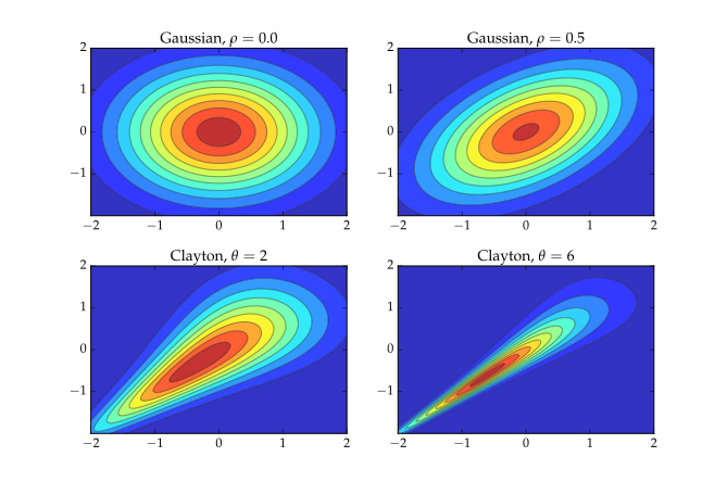
Copulas can be used to clarify a point raised in Section 5.1.3.2: normal marginals are not sufficient for the multivariate normal property. If $F_1, \ldots, F_N$ are univariate normal, then $C(F_1(s_1), \ldots, F_N(s_N))$ will equal the multivariate normal CDF for one choice of copula, called the Gaussian copula. Other choices lead to different distributions. Figure 5.5 gives an illustration where the top two distributions are multivariate normal and the bottom two are created by pairing the Clayton copula with univariate normal marginals. The distributions are represented as densities.

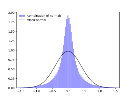
A related point is that while linear combinations of normal random variables are often thought to be normal, this isn’t true unless the original random variables are multivariate normal (cf., fact 5.1.5) or independent (which is a special case of multivariate normal). As an example, figure 5.6 shows a histogram of draws from $w = x-y$ when $(x,y)$ is distributed according to the density in the lower right panel of figure 5.5. For comparison, a normal density with the same mean and standard deviation is plotted.

5.1.6Properties of Named Distributions¶

Here are some useful facts relating independence and certain common distributions.

Let’s note some facts connecting chi-squared and normal random variables. First, if $\lL(x) = \nN(0, 1)$, then $\lL(x^2) = \chi^2(1)$. Exercise 5.4.4 asks you to prove this. Second, if a collection of standard normals are independent, then so are their squares (fact 5.1.10). Combining this result with fact 5.1.15 gives

The next result generalizes fact 5.1.18 and crops up frequently in statistics.

We can obtain fact 5.1.19 from fact 5.1.18 as follows. Since $\boldA$ is symmetric, we use the spectral decomposition theorem to write it as $\boldA = \boldQ \boldLambda \boldQ^\T$, where $\boldQ$ is an orthogonal matrix and $\boldLambda = \diag(\lambda_1, \ldots, \lambda_N)$ with $\lambda_n :=$ the $n$th eigenvalue of $\boldA$. Setting $\boldy := \boldQ^\T \boldz$, we have

By exercise 3.5.35, idempotence of $\boldA$ implies all eigenvalues lie in $\{0, 1\}$. By fact 3.2.7, the number of nonzero eigenvalues is equal to $\trace \boldA$. It follows that $\boldz^\T \boldA \boldz$ is the sum of $y^2_n$ over $K := \trace \boldA$ nonzero terms. By fact 5.1.18, a random variable with this property is $\chi^2(K)$ whenever $\boldy$ is standard normal. Combining $\lL(\boldz) = \nN(\boldzero, \boldI)$ and fact 5.1.5, we have $\lL(\boldy) = \nN(\boldzero, \boldQ^\T\boldQ)$. But $\boldQ$ is an orthogonal matrix, so $\boldQ^\T\boldQ = \boldI$.

5.2Conditioning and Expectation¶

Conditional expectation is one of the most important concepts in both economic theory and econometrics. This section gives a construction of expectation based around projection, which, in my view, is more intuitive and rewarding than both the elementary treatments using conditional distributions and the advanced treatments using Radon–Nykodym derivatives. The construction begins by formalizing the concepts of information and conditioning. We then build on our knowledge of orthogonal projection from Section 3.3 to frame conditional expectation as optimal prediction given limited information.

5.2.1Conditional Distributions¶

Let’s briefly discuss conditional distributions, focusing on the density case. Let $x_1$ and $x_2$ be random variables. The conditional density of $x_2$ given $x_1 = s_1$ is defined as

whenever the denominator is nonzero. Here $p$ stands in for either joint, marginal, or conditional density, with the type determined by the argument. (For example, $p(s_i)$ is the marginal density of $x_i$ evaluated at $s_i$.)

The law of total probability extends to the density case as follows: If $(x_1, x_2)$ is a random vector on $\RR^2$, then

To see this, fix $s_2 \in \RR$ and integrate the joint density to get the marginal, giving

Combining this result with $p(s_2 \given s_1) = p(s_1, s_2)/p(s_1)$ yields (5.24). Bayes’ law also extends to the density case, giving

The same ideas extend to additional arguments in a natural way. For example, the conditional density of $x_{k+1},\ldots, x_N$ given $x_1 = s_1,\ldots, x_k = s_k$ is defined by

Rearranging this expression, we obtain a useful decomposition of the joint density:

5.2.2The Space $L_2$¶

Suppose we want to predict random variable $y$ using another variable $x$. In this case we should choose $x$ such that $x$ and $y$ are expected to be close under most realizations of uncertainty. But what does "expected to be close" mean?

Perhaps the most common measure of distance between random variables is mean squared error (MSE), which is defined in this case as $\EE [ (x - y)^2 ]$. We met this concept previously in the linear prediction problem of Section 4.1.5. A common variation on MSE is root mean squared error, which, as the name suggests, is defined as

On the right-hand side of (5.28) we have a measure of distance between random variables. On the left-hand side we have used the same symbol as we used for Euclidean norm distance between two vectors. This is both deliberate and conventional, as there are many parallels between ordinary vector space with the Euclidean norm and the set of random variables combined with the "norm" defined in (5.28). Let’s now clarify and formalize these ideas.

The first geometric concept we defined for vectors was inner product. Analogously, we define here the inner product between two random variables $x$ and $y$ as

Of course we want this definition to make sense, and the Cauchy–Schwarz inequality for random variables tells us that $\EE[xy]$ will be finite and well-defined whenever $x$ and $y$ both have finite second moments. Hence we restrict attention to this set, which is commonly denoted $L_2$. That is,

Here’s a list of some of the ways that $L_2$ inner product is similar to the Euclidean inner product on $\RR^N$.

If you compare fact 5.2.1 with fact 2.1.1 you’ll see that the correspondence is essentially one-to-one. The properties in fact 5.2.1 follow from the definition of the inner product and linearity of $\EE$ (see fact 4.1.5).

Analogous to the Euclidean vector norm, we define the $L_2$ norm by

From this norm we get a notion of distance $\|x - y\|$ between random variables that agrees with the notion of root MSE in (5.28). As with inner product, the properties of the $L_2$ norm and vector norm are largely identical. (Compare the following with fact 2.1.2.)

Point (i) requires a clarification, which is given below. Property (ii) is immediate from (5.30) and the linearity of $\EE$. Property (iii) is called the triangle inequality, as in the vector case. Property (iv) is just the Cauchy–Schwarz inequality, restated in new notation. As in the vector case, the triangle inequality can be proved from the Cauchy–Schwarz inequality. For a proof, see exercise 5.4.15.

Returning to (i), it isn’t true that $\| x \| = 0$ implies $x(\omega) = 0$ for all $\omega \in \Omega$. What we can say is that if $\| x \| = 0$ then $\PP\{x =0\} =1$ (see, e.g., Williams (1991), §5.2). If we agree not to distinguish between random variables that only differ with zero probability, then (i) is valid. This is the standard convention when dealing with $L_2$.

5.2.2.1Linear Subspaces in $L_2$¶

From (ii) and (iii) of fact 5.2.2, we see that if $\alpha, \beta \in \RR$ and $x, y \in L_2$, then $\alpha x + \beta y$ also has finite norm, and is therefore in $L_2$. More generally, any linear combination

is again in $L_2$. As in the vector case (see Section 2.1.2), when $X$ is a subset of $L_2$, the set of finite linear combinations that can be formed from elements of $X$ is called the span of $X$, and denoted by $\Span X$.

A subset $S$ of $L_2$ is called a linear subspace of $L_2$ if it is closed under addition and scalar multiplication. That is, for each $x, y \in S$ and $\alpha, \beta \in \RR$, we have $\alpha x + \beta y \in S$.

As in $\RR^N$, an orthonormal basis of a linear subspace $S$ of $L_2$ is a set $\{u_1, \ldots, u_K\} \subset S$ with the property that

5.2.3Projections in $L_2$¶

Given that inner products and norms in $L_2$ share so many properties with their Euclidean cousins, it’s not surprising that many results about $\RR^N$ carry over to $L_2$. Often we can just lift the proofs across with barely a change to notation. We know a great deal about vectors and Euclidean space, so this process yields many insights about random variables. Let’s illustrate this in the context of orthogonal projection.

As in the Euclidean case, if $\inner{x,y}=0$, then we say that $x$ and $y$ are orthogonal, and write $x \perp y$. This terminology is used frequently in econometrics. Its importance stems partly from the next fact, the proof of which is a short exercise.

Now consider the following problem. Given $y \in L_2$ and linear subspace $S \subset L_2$, we seek the closest element $\hat y$ of $S$ to $y$. Closeness is in terms of $L_2$ norm, so $\hat y$ is the minimizer of $\| y - z \|$ over all $z \in S$. That is, we seek

The next theorem mimics theorem 2.2.1. A nice treatment that covers the current setting can be found in chapter 2 of Cheney (2001).

The statement that $S$ is closed means that $\{x_n \} \subset S$ and $x \in L_2$ with $\| x_n - x \| \to 0$ implies $x \in S$. This condition is true for all the linear subspaces we want to work with.

Analogous with the case of $\RR^N$, the random variable $\hat y$ in theorem 5.2.1 is called the orthogonal projection of $y$ onto $S$. Holding $S$ fixed, we can think of the operation

as a function from $L_2$ to $L_2$. The function will be denoted by $\boldP$, so that, for each $y \in L_2$, the symbol $\boldP y$ represents the image of $y$ under $\boldP$, which is the orthogonal projection $\hat y$. As before, $\boldP$ is called the orthogonal projection onto $S$, and we write $\boldP = \proj S$. Since $\boldP y$ solves (5.32), we can and do interpret $\boldP y$ as the best predictor of $y$ from within the collection of random variables contained in $S$.

Compare with theorem 2.2.2. In (i), the statement that $\boldP$ is linear means that $\boldP(\alpha x + \beta y) = \alpha \boldP x + \beta \boldP y$ for all $x, y \in L_2$ and $\alpha,\beta \in \RR$.

The next two results are $L_2$ versions of fact 2.2.7 and fact 2.2.6 respectively. The proofs are essentially the same.

5.2.3.1Population Regression¶

Let’s consider an extension of the best linear prediction problem of example 5.2.6 to a more general setting, where the information for predicting $y$ is a random vector $\boldx$ in $\RR^K$. As before, prediction will be linear, with the aim of minimizing squared error. Hence the object we seek is the $L_2$ orthogonal projection of $y$ onto the linear subspace

To make sure that $\Span\{\boldx\} \subset L_2$, we will assume that $\EE[ \boldx^\T \boldx] < \infty$.

Exercise 5.4.16 asks you to prove this. Positive definiteness of $\EE[\boldx \boldx^\T]$ ensures invertibility, without which the vector $\boldb^*$ is not uniquely defined (see ex. 3.5.34). Note that, by the definition of orthogonal projections, $\boldb^*$ necessarily satisfies

The linear prediction problem considered here is also called population linear regression. The "population" qualifier is because we are using the true joint distribution of $(\boldx, y)$ when we compute expectations. Population regression has a sample counterpart called multivariate linear regression, based on observations of $(\boldx, y)$. We will discuss it at length in chapter 11.

5.2.4Measurability¶

While the use of projections to obtain best linear predictors in example 5.2.6 and fact 5.2.7 is elegant and useful, we don’t always want to constrain ourselves to linear predictions. To drop the linearity requirement, we change the linear subspaces used for projection from the set of linear functions of $\boldx$ to the set of arbitrary functions of $\boldx$. As we now show, the best predictor that results is exactly the conditional expectation with respect to $\boldx$.

The key to this process is defining the subspace to project onto. In the language of probability, the subspace of arbitrary real-valued functions of $\boldx$ is called the $\boldx$-measurable functions. Let’s take these ideas one step at a time, starting with the notion of measurability with respect to information sets.

Let $\gG := \{x_1, \ldots, x_D\}$ be any set of random variables and let $z$ be any other random variable. The variable $z$ is said to be $\gG$-measurable if there exists a $\bB$-measurable function $g \colon \RR^D \to \RR$ such that

As usual, this equality between random variables should be interpreted pointwise, so the more explicit version is

In this context, $\gG$ is sometimes referred to as the information set. When convenient we’ll also write $\boldx = (x_1, \ldots, x_D)$ and say that $z$ is $\boldx$-measurable. Similar terminology will be used for scalars and matrices. For example, if $\boldX$ is a random matrix, then $\boldX$-measurability means $\gG$-measurability when $\gG$ lists all elements of $\boldX$.

The intuitive meaning of $\gG$-measurability of $z$ is that $z$ is completely determined by the elements in $\gG$. Imagine it like this: When uncertainty is realized, some $\omega$ is selected from $\Omega$. We don’t get to view $\omega$ itself, but we do get to observe the realized values $x_1(\omega), \ldots, x_D(\omega)$ on the right-hand side of (5.36). If $z$ is $\gG$-measurable, we can now calculate the realized value $z(\omega)$ of $z$, even without knowing $\omega$.