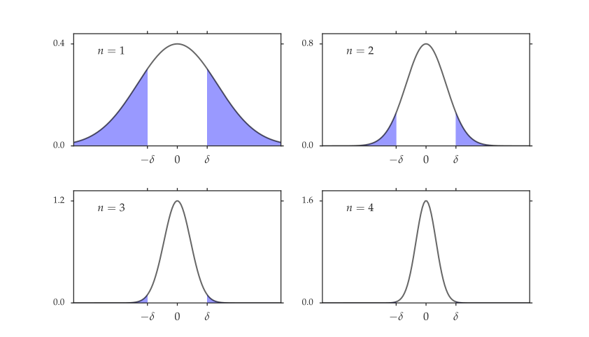
The law of large numbers and central limit theorem are two of the pillars of econometrics and statistics. Below we review both theorems, starting with the necessary concepts of convergence in probability and distribution.
Part (i) is an immediate consequence of the definition. Other proofs are touched on in the exercises. For more details, see, for example, Çinlar (2011).
The scalar sequence {xn} is said to converge to xin mean square if
and we write xn→msx. Unlike convergence in probability, for convergence in mean square to be defined we require that our variables have finite second moments.
Part (i) follows from Chebyshev’s inequality . In particular, from monotonicity of P and (4.19) we get
P{∣xn−x∣>δ}⩽P{∣xn−x∣⩾δ}⩽δ2E(xn−x)2
Part (ii) is implied by the next fact.
As we’ll see later, (6.3) plays an important role in statistics. Its verification is an exercise. (The proof is straightforward. If you want more of a challenge, try to obtain it as a consequence of (iv) of fact 5.2.4.)
The law of large numbers (LLN) is one of the most fundamental theorems of both probability and statistics. As a prelude to the LLN, let’s consider the effects of averaging over independent random quantities. We’ll take the perspective of investors, who often diversify their portfolios in order to decrease risk. To formalize this idea let
xn be the payoff from holding one dollar of asset n,
Exn=μ and var[xn]=σ2 for all n, and
cov[xj,xk]=0 when j=k.
If we hold just asset 1, then the payoff is x1, the expected payoff is μ and the variance is σ2. If we diversify by spreading one dollar evenly over N of these assets, our payoff is
The important equality here is the third one, which holds because of the zero covariance between assets. In this step N2 terms become N terms. To summarize,
Now imagine someone is kind enough to sell us an unlimited quantity of such assets, so we can diversify without limit. By taking N→∞ and combining (6.5) with fact 6.1.2 we obtain a proof of the law of large numbers:
Actually we haven’t fully proved the LLN because we assumed existence of second moments above, while theorem 6.1.1 assumes only existence of the first moment. However, the proof above captures the spirit of the LLN most cleanly. (See theorem 8.3.5 of Dudley(2002) for the general case.)
At first glance, the law of large numbers (6.6) appears to only be a statement about the sample mean but in fact it’s self-improving: We can go from (6.6) to arbitrary functions of random variables, or even random vectors. In particular, if x is any random vector, {xn} are IID copies and h:RN→R is any B-measurable function such that h(x) is integrable, then
This can be confirmed by letting yn:=h(xn) and then applying theorem 6.1.1. The independence of {yn} is confirmed by fact 5.1.10. That each yn has the same distribution as y:=h(x) follows from
P{yn∈B}=P{h(xn)∈B}=P{xn∈h−1(B)}=P{x∈h−1(B)}
The law of large numbers applies to probabilities as well as expectations. To see this, fix B⊂B(RN), and consider the probability P{x∈B}. Letting h be the indicator function h(s)=11B(s)=11{s∈B} and using the principle that expectations of indicators equal probabilities of events, we have
Eh(x)=E11{x∈B}=P{x∈B}
Combining this equality with (6.7), we see that if {xn} is IID with distribution P, then
To illustrate the law of large numbers, consider flipping a coin until 10 heads have occurred. The coin is not fair: The probability of heads is 0.4. Let x be the number of tails observed in the process. This random variable is known to have the negative binomial distribution, with Ex=15. The LLN predicts that if we simulate a large number of observations of x and take the average, we get a value close to 15. Running the Julia code in listing 1 gives outcomes consistent with this claim.[1]
num_reps = 10^6
outcomes = Vector{Float64}(undef, num_reps)

for i in 1:num_reps
    num_tails = num_heads = 0
    while num_heads < 10
        b = rand()
        num_heads = num_heads + (b < 0.4)   # +1 with prob 0.4
        num_tails = num_tails + (b >= 0.4)  # +1 with prob 0.6
    end
    outcomes[i] = num_tails
end

println(sum(outcomes) / num_reps)
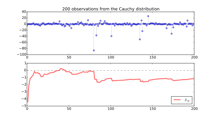
Figure 6.2 shows what can happen when the finite first moment condition in the LLN is not enforced. The draws are from the standard Cauchy distribution, which fails to have a finite first moment. The top panel shows observations and the bottom shows a running sample mean of observations xˉN, with N on the horizontal axis. A few extreme observations dominate the average and the sample mean does not converge.[2]
Figure 6.2:Samples from the Cauchy distribution and sample mean
As a prelude to the central limit theorem we need to review convergence in distribution. This is conceptually quite different to convergence of random variables, whether in probability or mean square. For example, the distributions N(0,1) and N(10−10,1) are very close, but independent draws from these respective distributions need not be.
Let {Pn} and P be distributions on RK in the sense of Section 5.1.2. To represent the notion that Pn converges to P we could require that Pn(B)→P(B) for all B∈B(RK). However, this turns out to be rather strict and also indifferent to closeness in the sense of Euclidean norm. For example, suppose that Pn is a distribution on R that puts all mass on n1, while P puts all mass on 0. Intuition suggests that Pn→P, but if we take B=(0,∞), we have Pn(B)=1 for all n, while P(B)=0.
For this reason the common notion of convergence of distributions, which is called weak convergence, requires only that Pn(B)→P(B) for all "continuity sets" in RK. There’s an equivalent way to phrase this that’s easier to work with in applications: We say that {Pn}converges weakly to P if
∫h(s)Pn(ds)→∫h(s)P(ds)for all continuous bounded h:RK→R
and write Pn→wP. For the definition of these integrals see Section 5.1.3.3. Continuity of h enforces respect for the topology on RK, while boundedness is imposed only to ensure that the integrals are finite.
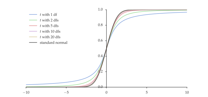
Figure 6.3:t-Distribution with k df converges to N(0,1) as k→∞
Sometimes densities are easier to work with than CDFs. In this connection, the following sufficient condition can be useful.
Let {xn} and x be random vectors. We say that xn→xin distribution if their respective distributions converge weakly. This convergence is symbolized by xn→dx. Thus
E[h(xn)]→E[h(x)]for all continuous bounded h:RK→R
Part (i) of fact 6.1.6 is called the continuous mapping theorem. Part (ii) is called the Cramér–Wold theorem, or the Cramér–Wold device. The next result is sometimes known as Slutsky’s theorem.
The central limit theorem is among the most striking and important results in all of mathematics. Relative to the LLN, it requires an additional second moment condition. Here’s a statement of the theorem in the scalar IID case.
The meaning of →d here is that the distribution of the left-hand side →wN(0,σ2). We can interpret (6.9) as follows: On one hand, (xˉN−μ)→p0 by the LLN; on the other, N→∞. If we take the product, these two competing terms just balance. Remarkably, the distribution of the product approaches a zero-mean Gaussian as N→∞, regardless of the distribution of x.
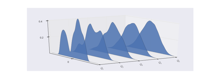
We’ll skip the proof of the CLT (which provides little intuition) and turn to simulation. For starters, see figure 6.4, where QN:= the distribution of the left-hand side of (6.9) for N=1,…,5. The initial distribution Q=Q1 is multi-modal, and was constructed as a convex combination of three beta distributions. The CLT predicts that QN→wN(0,σ2), where σ2=∫s2Q1(ds). Note how quickly the bell shape emerges, despite the irregularity of the initial distribution.
Figure 6.4:CLT in action, starting from a beta mixture
Another common statement of the central limit theorem is as follows: If all the conditions of theorem 6.1.2 are satisfied, then
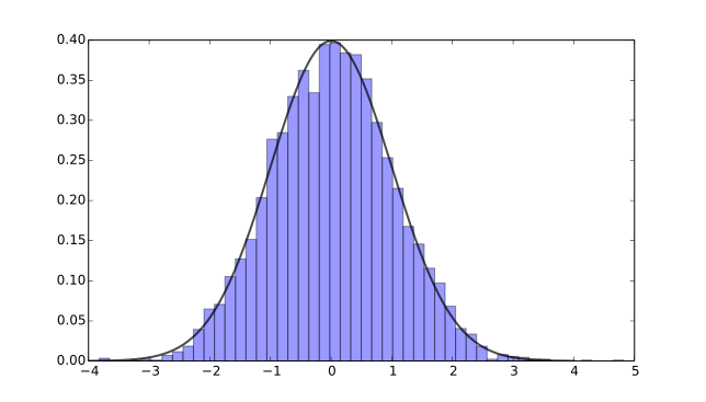
The convergence in (6.10) is illustrated by listing 2, the output of which is given in figure 6.5. The listing generates 5,000 observations of the random variable zN defined in (6.10), where each xn is χ2(5). (The mean of this distribution is 5, and the variance is 2×5=10.) The observations of zN are stored in the vector outcomes. The figure histograms this vector and then superimposes the density of the N(0,1) distribution.
import numpy as np
import scipy.stats as st

num_reps = 5000
outcomes = np.empty(num_reps)
N, k = 1000, 5     # k = degrees of freedom
chi = st.chi2(k)

for i in range(num_reps):
    xvec = chi.rvs(N)
    outcomes[i] = np.sqrt(N / (2 * k)) * (xvec.mean() - k)

# code to histogram outcomes and plot st.norm.pdf
# for comparison is omitted here
The notion of convergence in probability discussed in Section 6.1.1 extends naturally to matrices. Let {Xn}n=1∞ be a sequence of random N×K matrices. We say that Xn converges to a random N×K matrix Xin probability and write Xn→pX if
∥Xn−X∥→p0asn→∞
where ∥⋅∥ is the matrix norm defined in Section 3.3.5.
In part (iii) of fact 6.2.1, the matrices An and A are nonrandom and convergence is in matrix norm. Note that part (v) can be obtained from two applications of part (iii).
In econometrics we often use the vector version of Slutsky’s theorem:
The scalar LLN and CLT that we discussed above extend to the vector case in a natural way. For example,
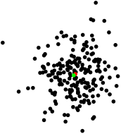
Here N1∑n=1Nxn should be understood in terms of vector addition and scalar multiplication. Thus xˉN is a convex combination of the sample points in RK. Figure 6.6 illustrates this in two dimensions. The green dot is μ. The black dots are realizations of x1,…,xN. The red dot is the sample mean N1∑n=1Nxn. By (6.11), the red dot converges to the green dot.
The vector LLN in theorem 6.2.1 follows from the scalar LLN. To see this, let xn be as in theorem 6.2.1, let a be any constant vector in RK, let yn:=a⊺xn and let y:=a⊺x. The sequence {yn} is IID (see fact 5.1.10) with the same distribution as y. By the scalar LLN (theorem 6.1.1), we have
The vector CLT in theorem 6.2.1 also follows from the scalar case and the proof is quite similar. See exercise 6.4.10.
These results can be further extended to random matrices. In fact we will need a matrix LLN in our investigation of linear regression. Here’s a suitable result:
The proof is straightforward: By fact 6.2.1, to prove (6.13), it suffices to show that N1∑n=1NXna→pE[X]a for any conformable vector a. Since Xna is a vector with expectation E[X]a, this is immediate from the vector LLN in theorem 6.2.1.
The asymptotic normality result in the central limit theorem is preserved under linear transformations, as follows from fact 6.2.2. It turns out that the same thing is true even for functions that are only locally almost linear—that is, for differentiable functions. This greatly extends the power and reach of the central limit theorem.
Here ∇g(θ) is the gradient vector of g at θ, which is defined as
In statistical settings, the technique of obtaining asymptotic distributions by appealing to theorem 6.2.2 is called the delta method. We will see its importance later on. The proof of theorem 6.2.2 is based on a Taylor expansion of g around the point θ. See theorem 3.1 of Vaart (2000). Exercise 6.4.9 walks you through some of the key ideas.
For high quality treatments of the law of large numbers and the central limit theorem see, for example, Dudley (2002), Taylor (1997), Durrett (2010), Pollard (2002), DasGupta (2008), or Çinlar (2011). An advanced but thorough treatment of the delta method can be found in Vaart (2000).
A routine to draw from the negative binomial distribution is available from the Distributions package, but we’ve rolled our own for extra transparency.