Vector Spaces - A Primer in Econometric Theory

Our first technical topic for this book is linear algebra, which is one of the foundation stones of applied mathematics in general, and econometrics and statistics in particular. Data ordered by observation are naturally stored in vectors. Related vectors are naturally grouped into matrices. Once our data are organized this way, we need to perform basic arithmetic operations or solve equations or quadratic minimization problems. In this chapter we cover the foundations of vector operations used in linear algebra. As we’ll see, the conceptual aspects of linear algebra are clearest if we begin by stripping away details such as matrices and look instead at linear operations from a more abstract perspective.

2.1Vectors and Vector Space¶

Let’s begin with vector space and basic vector operations.

2.1.1Vectors¶

For arbitrary $N \in \NN$ , the symbol $\RR^N$ represents the set of all $N$ -vectors, or vectors of length $N$ . A typical element has the form

\boldx = \left( \begin{array}{c} x_1 \\ x_2 \\ \vdots \\ x_N \end{array} \right) \quad \text{ where } x_n \in \RR \text{ for each } n

( $\RR = \RR^1$ represents the set of all real numbers, which is the union of the rational and irrational numbers.) While $\boldx$ has been written vertically, as a column of numbers, we could also write it horizontally as $\boldx = (x_1, \ldots, x_N)$ . For now vectors are just a sequences of numbers, and it makes no difference whether we write them vertically or horizontally. (Only when we work with matrix multiplication does it become necessary to distinguish between column and row vectors.)

The vector of ones will be denoted $\boldone$ and the vector of zeros will be denoted $\boldzero$ :

\boldone := \left( \begin{array}{c} 1 \\ \vdots \\ 1 \end{array} \right), \quad \quad \boldzero := \left( \begin{array}{c} 0 \\ \vdots \\ 0 \end{array} \right)

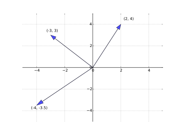
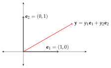
Although vectors are infinitesimal points in $\RR^N$ , they are often represented visually as arrows from the origin to the point itself. Figure 2.1 gives an illustration for the case $N=2$ .

Three vectors in \RR^2 — Figure 2.1:Three vectors in $\RR^2$

In vector space theory there are two fundamental algebraic operations: vector addition and scalar multiplication. For $\boldx, \boldy \in \RR^N$ , their vector sum is

\boldx + \boldy = \left( \begin{array}{c} x_1 \\ \vdots \\ x_N \end{array} \right) + \left( \begin{array}{c} y_1 \\ \vdots \\ y_N \end{array} \right) := \left( \begin{array}{c} x_1 + y_1 \\ \vdots \\ x_N + y_N \end{array} \right)

If $\alpha \in \RR$ , then the scalar product of $\alpha$ and $\boldx$ is defined to be

\alpha \boldx = \alpha \left( \begin{array}{c} x_1 \\ \vdots \\ x_N \end{array} \right) := \left( \begin{array}{c} \alpha x_1 \\ \vdots \\ \alpha x_N \end{array} \right)

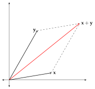
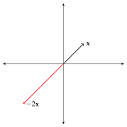
Thus addition and scalar multiplication are defined in terms of ordinary addition and multiplication in $\RR$ , computed element by element, adding and multiplying respectively.^[1] Figure 2.2 and Figure 2.3 show examples of vector addition and scalar multiplication in the case $N=2$ .

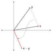
Subtraction of two vectors is performed element by element, just like addition. Subtraction is not a primitive operation because the definition can be given in terms of addition and scalar multiplication: $\boldx - \boldy := \boldx + (-1) \boldy$ . An illustration of subtraction is given in figure 2.4. One way to remember this operation is to draw a line from $\boldy$ to $\boldx$ and then shift it to the origin.

The inner product of two vectors $\boldx$ and $\boldy$ in $\RR^N$ is denoted by $\inner{\boldx, \boldy}$ , and defined as the sum of the products of their elements:

\inner{\boldx, \boldy} := \sum_{n=1}^N x_n y_n

(2.1)

These properties are easy to check from (2.1). For example, regarding the second equality, pick any $\alpha, \beta \in \RR$ and any $\boldx, \boldy \in \RR^N$ . By the definitions of scalar multiplication and inner product respectively, we have

\inner{\alpha \boldx, \beta \boldy} = \sum_{n=1}^N \alpha x_n \beta y_n = \alpha \beta \sum_{n=1}^N x_n y_n = \alpha \beta \inner{\boldx, \boldy}

The (Euclidean) norm of a vector $\boldx \in \RR^N$ is defined as

\| \boldx \| := \sqrt{\inner{\boldx, \boldx}}

(2.2)

and represents the length of the vector $\boldx$ . (In the arrow representation of vectors in figures 2.2–2.4, the norm of the vector is equal to the length of the arrow.)

Properties (i) and (ii) you can verify yourself without difficulty. Proofs for (iii) and (iv) are a bit harder. Property (iii) is called the triangle inequality, while (iv) is called the Cauchy–Schwarz inequality. The proof of the Cauchy–Schwarz inequality is given as a solved exercise after we’ve built up some more tools (see ex. 3.5.33). If you’re prepared to accept the Cauchy–Schwarz inequality for now, then the triangle inequality follows, because, by the properties of the inner product given in fact 2.1.1,

\| \boldx + \boldy \|^2 = \inner{\boldx + \boldy, \boldx + \boldy} = \inner{\boldx, \boldx} + 2 \inner{\boldx, \boldy} + \inner{\boldy, \boldy} \leq \inner{\boldx, \boldx} + 2 | \! \inner{\boldx, \boldy} \! | + \inner{\boldy, \boldy}

Given two vectors $\boldx$ and $\boldy$ , the value $\| \boldx - \boldy \|$ has the interpretation of being the “distance” between these points. To see why, consult figure 2.4 again.

2.1.2Linear Combinations and Span¶

One of the most elementary ways to work with vectors is to combine them using linear operations. Given vectors $\boldx_1,\ldots, \boldx_K$ in $\RR^N$ , a linear combination of these vectors is a new vector of the form

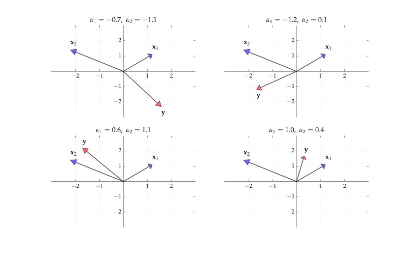
\boldy = \sum_{k=1}^K \alpha_k \boldx_k = \alpha_1 \boldx_1 + \cdots + \alpha_K \boldx_K

(2.3)

for some collection of scalars $\alpha_1,\ldots, \alpha_K$ (i.e., with $\alpha_k \in \RR$ for all $k$ ). Figure 2.5 shows four different linear combinations $\boldy = \alpha_1 \boldx_1 + \alpha_2 \boldx_2$ where $\boldx_1, \boldx_2$ are fixed vectors in $\RR^2$ and the scalars $\alpha_1$ and $\alpha_2$ are varied.

Linear combinations of \boldx_1, \boldx_2 — Figure 2.5:Linear combinations of $\boldx_1, \boldx_2$

Given any nonempty $X \subset \RR^N$ , the set of all vectors that can be made by (finite) linear combinations of elements of $X$ is called the span of $X$ , and denoted by $\Span X$ . For example, the set of all linear combinations of $X := \{\boldx_1,\ldots, \boldx_K\}$ is

\Span X:= \left\{ \text{ all vectors } \sum_{k=1}^K \alpha_k \boldx_k \text{ such that } \boldalpha := (\alpha_1,\ldots, \alpha_K) \in \RR^K \right\}

As will be discussed below, the span of certain collections of vectors turns out to have an intimate connection with existence of solutions to linear equations.

Span of X = \{\boldx_1, \boldx_2\} — Figure 2.6:Span of $X = \{\boldx_1, \boldx_2\}$

Example 2.1.4

Consider the vectors $\{\bolde_1, \ldots, \bolde_N\} \subset \RR^N$ , where $\bolde_n$ has all zeros except for a $1$ as the $n$ th element:

\bolde_1 := \left( \begin{array}{c} 1 \\ 0 \\ \vdots \\ 0 \end{array} \right), \quad \bolde_2 := \left( \begin{array}{c} 0 \\ 1 \\ \vdots \\ 0 \end{array} \right), \quad \cdots, \quad \bolde_N := \left( \begin{array}{c} 0 \\ 0 \\ \vdots \\ 1 \end{array} \right)

The case of $\RR^2$ is illustrated in figure 2.7. The vectors $\bolde_1, \ldots, \bolde_N$ are called the canonical basis vectors of $\RR^N$ . One reason is that $\{\bolde_1, \ldots, \bolde_N\}$ spans all of $\RR^N$ . Here’s a proof for $N=2$ : Observe that for any $\boldy \in \RR^2$ , we have

\boldy := \left( \begin{array}{c} y_1 \\ y_2 \end{array} \right) = \left( \begin{array}{c} y_1 \\ 0 \end{array} \right) + \left( \begin{array}{c} 0 \\ y_1 \end{array} \right) = y_1 \left( \begin{array}{c} 1 \\ 0 \end{array} \right) + y_2 \left( \begin{array}{c} 0 \\ 1 \end{array} \right) = y_1 \bolde_1 + y_2 \bolde_2

Thus $\boldy \in \Span \{\bolde_1, \bolde_2\}$ . Since $\boldy$ is an arbitrary vector in $\RR^2$ , we have shown that $\{\bolde_1, \bolde_2\}$ spans $\RR^2$ .

Canonical basis vectors in \RR^2 — Figure 2.7:Canonical basis vectors in $\RR^2$

The next fact follows directly from the definition of span.

2.1.3Linear Independence¶

Linear independence is an apparently simple concept with implications that stretch deep into many aspects of analysis. If you wish to understand when a matrix is invertible, or when a system of linear equations has a unique solution, or when a least squares estimate is uniquely defined, the most important foundational idea is linear independence of vectors.

Let’s begin with the definition. Consider a set of vectors $X := \{\boldx_1,\ldots, \boldx_K\}$ . We can surely realize the origin $\boldzero$ as a linear combination of these vectors, just by setting all of the scalars $\alpha_k$ in $\sum_{k=1}^K \alpha_k \boldx_k$ to zero. The set $X$ is called linearly independent when this is the only possibility. That is, $X \subset \RR^N$ is called linearly independent if

\alpha_1 \boldx_1 + \cdots + \alpha_K \boldx_K = \boldzero \quad \implies \quad \alpha_1 = \cdots = \alpha_K = 0

(2.4)

We call $X$ linearly dependent if it is not linearly independent.

Example 2.1.6

In figure 2.5, the two vectors are $\boldx_1 = (1.2, 1.1)$ and $\boldx_2 = (-2.2, 1.4)$ . Suppose that $\alpha_1$ and $\alpha_2$ are scalars with

\alpha_1 \left( \begin{array}{c} 1.2 \\ 1.1 \end{array} \right) + \alpha_2 \left( \begin{array}{c} -2.2 \\ 1.4 \end{array} \right) = \boldzero

This translates to the linear, two-equation system shown in figure 2.8, where the unknowns are $\alpha_1$ and $\alpha_2$ . The only solution is $\alpha_1 = \alpha_2 = 0$ . Hence $\{\boldx_1, \boldx_2\}$ is linearly independent.

The only solution is \alpha_1 = \alpha_2 = 0 — Figure 2.8:The only solution is $\alpha_1 = \alpha_2 = 0$

Example 2.1.7

The set of $N$ canonical basis vectors $\{\bolde_1, \ldots, \bolde_N\}$ is linearly independent in $\RR^N$ . To see this, let $\alpha_1, \ldots, \alpha_N$ be coefficients such that $\sum_{n=1}^N \alpha_n \bolde_n = \boldzero$ . Equivalently,

\alpha_1 \left( \begin{array}{c} 1 \\ 0 \\ \vdots \\ 0 \end{array} \right) + \alpha_2 \left( \begin{array}{c} 0 \\ 1 \\ \vdots \\ 0 \end{array} \right) + \cdots + \alpha_N \left( \begin{array}{c} 0 \\ 0 \\ \vdots \\ 1 \end{array} \right) = \left( \begin{array}{c} \alpha_1 \\ \alpha_2 \\ \vdots \\ \alpha_N \end{array} \right) = \left( \begin{array}{c} 0 \\ 0 \\ \vdots \\ 0 \end{array} \right)

In particular, $\alpha_n = 0$ for all $n$ .

How can we interpret linear independence? One way to understand it is as an indicator of the algebraic diversity of a given collection of vectors. In particular, in a linearly independent set, the span is relatively large, in the sense that every vector contributes to the span. Here’s a formal statement of this idea.

Exercise 2.4.15 asks you to check these equivalences. For now let’s just step through them in the context of two examples. First consider the pair of canonical basis vectors $\{\bolde_1, \bolde_2\}$ in $\RR^2$ , as depicted in figure 2.7. As we saw in examples 2.1.4 and 2.1.7, this pair is linearly independent, and its span is all of $\RR^2$ . Both vectors contribute to the span, since removing either one reduces the span to just a line in $\RR^2$ . (For example, the span of $\{\bolde_1\}$ is just the horizontal axis in $\RR^2$ .) Neither one of this pair can be written as a linear combination of the other.

Next, consider instead the pair $\{\boldx_1, \boldx_2\}$ in example 2.1.8. These vectors fail to be linearly independent, as shown in that example. It is also clear that dropping either one does not change the span—it remains the horizontal axis in any case. Finally, we saw in example 2.1.8 that $\boldx_2 = -2 \boldx_1$ , which means that each vector can be written as a linear combination of the other.

The proof is a solved exercise (ex. 2.4.16).

2.1.3.1Linear Independence and Uniqueness¶

As we’ll see below, the problem of existence of solutions to systems of linear equations comes down to whether or not a given point is contained in the span of a collection of vectors (which typically correspond to the columns of a matrix). This depends in general on the size of the span, and the size of the span in turn depends on whether or not the vectors are linearly independent.

Given that linear independence is the key condition for existence of solutions, it’s surprising at first to learn that linear independence is the key condition for uniqueness as well. As we’ll see, the connection between linear independence and uniqueness stems from the following result.

Proof

((i) $\implies$ (ii)) Let $X$ be linearly independent and pick any $\boldy \in \RR^N$ . Suppose that there are two sets of scalars such that (2.5) holds. In particular, suppose that $\boldy = \sum_{k=1}^K \alpha_k \boldx_k = \sum_{k=1}^K \beta_k \boldx_k$ . It follows from the second equality that $\sum_{k=1}^K (\alpha_k - \beta_k) \boldx_k = \boldzero$ . By linear independence, we then have $\alpha_k = \beta_k$ for all $k$ . In other words, the representation is unique.

((ii) $\implies$ (i)) If (ii) holds, then there exists at most one set of scalars such that $\boldzero = \sum_{k=1}^K \alpha_k \boldx_k$ . Because $\alpha_1 = \cdots = \alpha_k = 0$ has this property, we conclude that no nonzero scalars yield $\boldzero = \sum_{k=1}^K \alpha_k \boldx_k$ . In other words, $X$ is linearly independent. ◻

2.1.4Linear Subspaces¶

We will find it rewarding to study more closely the structure of spans generated by a collection of vectors. One of the defining features of the span of a set $X$ is that it is “closed” under the linear operations of vector addition and scalar multiplication, in the sense that

$\boldx, \boldy \in \Span X \; \implies \; \boldx + \boldy \in \Span X$ , and
$\boldy \in \Span X$ and $\gamma \in \RR \; \implies \; \gamma \boldy \in \Span X$ .

For example, (i) holds because the sum of two linear combinations of elements of $X$ is another linear combination of elements of $X$ .

The notion of a set being closed under scalar multiplication and vector addition is important enough to have its own name: A nonempty subset $S$ of $\RR^N$ is called a linear subspace (or just subspace) of $\RR^N$ if

\boldx, \, \boldy \in S \text{ and } \alpha, \, \beta \in \RR \; \implies \; \alpha \boldx + \beta \boldy \in S

(2.6)

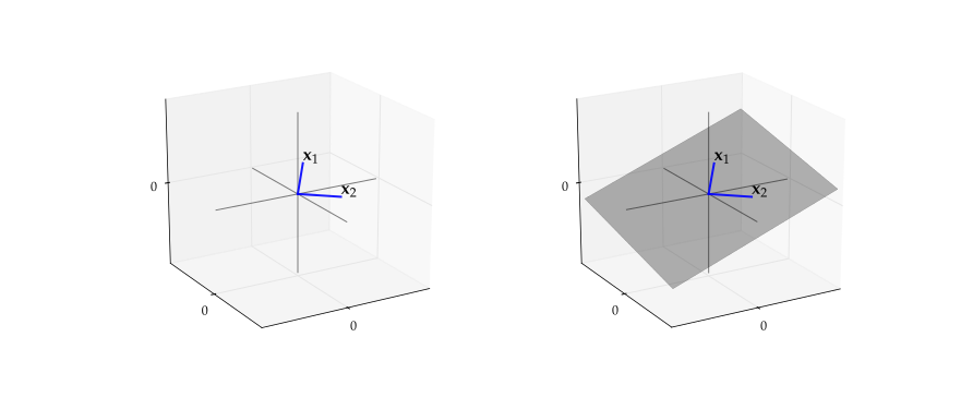
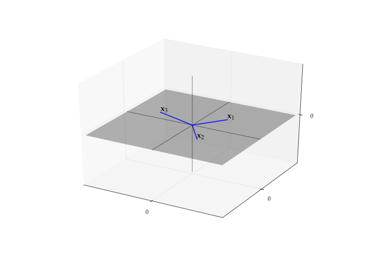
To visualize subspaces in $\RR^3$ , think of lines and planes that pass through the origin. Here are some elementary facts about linear subspaces:

There’s also one deep result about linear subspaces we need to cover, which forms a cornerstone of many foundational results:

In other words, if there exists a set $X = \{\boldx_1, \ldots, \boldx_K\}$ with $S \subset \Span X$ , then any subset of $S$ with more than $K$ vectors will be linearly dependent. The proof can be found in most texts on linear algebra (e.g., §3.5 of Jänich (1994)).

Any three vectors in P are linearly dependent — Figure 2.9:Any three vectors in $P$ are linearly dependent

2.1.5Bases and Dimension¶

Consider again the pair $\boldx_1, \boldx_2$ shown in figure 2.5, and the four different vectors labeled $\boldy$ that we created from $\boldx_1, \boldx_2$ by way of linear combinations. Eyeballing the figure gives the impression that any $\boldy \in \RR^2$ could be constructed as a linear combination of $\boldx_1, \boldx_2$ with suitable choice of the scalars $\alpha_1, \alpha_2$ . Indeed this is true. The reason is that the pair $\{\boldx_1, \boldx_2\}$ is linearly independent (see example 2.1.6), and any pair of linearly independent vectors in $\RR^2$ spans $\RR^2$ . Here’s a statement of this result for the general case:

Proof

((i) $\implies$ (ii)) Suppose that $\Span X = \RR^N$ but $X$ is not linearly independent. Then, by theorem 2.1.1, there exists a proper subset $X_0$ of $X$ with $\Span X_0 = \Span X$ . Since $X_0$ is a proper subset of $X$ it contains $K < N$ elements. We now have $K$ vectors spanning $\RR^N$ . In particular, the span of $K$ vectors contains the $N>K$ linearly independent vectors $\bolde_1, \ldots, \bolde_N$ . This contradicts theorem 2.1.3.

((ii) $\implies$ (i)) Suppose that $X$ is linearly independent and yet there exists an $\boldx \in \RR^N$ with $\boldx \notin \Span X$ . By fact 2.1.4, it follows that the $N+1$ element set $X \cup \{\boldx\} \subset \RR^N$ is linearly independent. Since $\RR^N$ is spanned by the $N$ canonical basis vectors, this statement also contradicts theorem 2.1.3. ◻

We now come to a key definition. Let $S$ be a linear subspace of $\RR^N$ and let $B \subset S$ . The set $B$ is called a basis of $S$ if

$B$ spans $S$ and
$B$ is linearly independent.

The plural of basis is bases. In view of theorem 2.1.2, when $B$ is a basis of $S$ , each point in $S$ has exactly one representation as a linear combination of elements of $B$ .

It follows immediately from theorem 2.1.4 that any $N$ linearly independent vectors in $\RR^N$ form a basis of $\RR^N$ .

Here are the two most fundamental results about bases:

The proof of part (i) is not particularly hard. See, for example, section 3.2 of Jänich (1994). Part (ii) follows from theorem 2.1.3 and is left as an exercise (ex. 2.4.17).

If $S$ is a linear subspace of $\RR^N$ , then the common number identified in theorem 2.1.5 is called the dimension of $S$ , and written as $\dim S$ .

In $\RR^N$ the singleton subspace $\{\boldzero\}$ is said to have zero dimension.

If we take a set of $K$ vectors, then how large will its span be in terms of dimension? The next theorem answers this question.

Exercise 2.4.19 asks you to prove these results.

Let’s finish this section with facts that can be deduced from the preceding results.

Part (i) of fact 2.1.6 implies that the only $N$ -dimensional linear subspace of $\RR^N$ is $\RR^N$ itself.

2.1.6Linear Maps¶

The single most important class of functions in applied mathematics is the linear functions. In high school we are told that linear functions as those whose graph is a straight line. Here’s a better definition: A function $T \colon \RR^K \to \RR^N$ is linear if

T(\alpha \boldx + \beta \boldy) = \alpha T\boldx + \beta T\boldy \; \text{ for any } \boldx, \boldy \in \RR^K \text{ and } \alpha, \beta \in \RR

(2.7)

(Following a common convention, we’ll write linear functions with uppercase letters and omit the parenthesis around the argument where no confusion arises. This convention has come about because the action of linear maps is essentially isomorphic to multiplication of vectors by matrices. More on that topic soon.)

The definition in (2.7) tells us directly that if $T$ is linear then the exchange of order in $T [ \sum_{k=1}^K \alpha_k \boldx_k ] = \sum_{k=1}^K \alpha_k T \boldx_k$ will be valid whenever $K=2$ . A simple inductive argument extends this to arbitrary $K$ . As an application of this fact, consider the following: As discussed in example 2.1.4, any $\boldx \in \RR^K$ can be expressed in terms of the basis vectors as $\sum_{k=1}^K \alpha_k \bolde_k$ , for some suitable choice of scalars. Hence, for a linear function $T$ , its range, denoted $\range T$ , is the set of all points of the form

T\boldx = T \left[ \sum_{k=1}^K \alpha_k \bolde_k \right] = \sum_{k=1}^K \alpha_k T \bolde_k

as we vary $\alpha_1, \ldots, \alpha_K$ over all scalar combinations. (See Section 15.2 for the definition of range.) In other words, the range of a linear map is the span of the image of the canonical basis functions. This will prove to be important later on. The next fact summarizes.

Soon we’ll turn to the topic of determining when linear functions are bijections, an issue that is intimately related to invertibility of matrices. To this end it’s useful to note that, for linear functions, the property of being one-to-one can be determined by examining the set of points it maps to the origin. To express this idea, for any $T \colon \RR^K \to \RR^N$ , we define the null space or kernel of $T$ as

\kernel T := \setntn{\boldx \in \RR^K}{T\boldx = \boldzero}

The proofs are straightforward. For example, if $T\boldx = T\boldy$ for some $\boldx, \boldy \in \RR^K$ , then $T(\boldx - \boldy) = \boldzero$ , and hence $\boldx - \boldy \in \kernel T$ . So if $\kernel T = \{\boldzero\}$ , then $T\boldx = T\boldy$ implies $\boldx = \boldy$ , which means that $T$ is one-to-one.

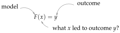
2.1.7Linear Independence and Bijections¶

Many statistical problems are "inverse" problems, in the sense that we observe outcomes and wish to determine what generated them. For example, we might want to know what consumer preferences led to observed market behavior, or what kinds of expectations led to a given shift in exchange rates.

Consider the generic inverse problem in figure 2.10, where $F$ and $y$ are given, and we seek to obtain the unknown object $x$ . Two immediate questions are: Does this problem have a solution? and Is it unique? To provide general answers to these questions, we need to know whether $F$ is one-to-one, onto, etc. (see Section 15.2 for definitions and further discussion). The best case is when $F$ is a bijection, for then we know that a unique solution $x$ exists for every possible $y$ .

In general, functions can be onto, one-to-one, bijections, or none of the above. However, for linear functions from $\RR^N$ to $\RR^N$ , the first three properties are all equivalent! The next theorem gives details.

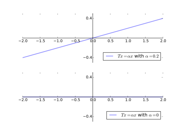
If any one of these conditions is true, then $T$ is called nonsingular. (Equivalently, a nonsingular function is a linear bijection.) Otherwise $T$ is called singular. The proof of theorem 2.1.7 is a solved exercise (ex. 2.4.21). Figure 2.11 provides intuition for the case of $N=1$ . In the top panel all conditions in theorem 2.1.7 are satisfied. In the lower panel none are. In particular, we can see that the condition for $T$ to be one-to-one and onto is exactly the same (i.e., $\alpha \neq 0$ ).

The case of N=1, nonsingular and singular — Figure 2.11:The case of $N=1$ , nonsingular and singular

If $T$ is nonsingular, then, being a bijection, it must have an inverse function $T^{-1}$ that is also a bijection (fact 15.2.1). It turns out that this inverse function inherits the linearity of $T$ (see ex. 2.4.20). In summary,

Theorem 2.1.7 only applies to linear maps between spaces of the same dimension. When linear functions map across distinct dimensions the situation changes:

The most important implication is that if $N \neq K$ , then we can forget about bijections. The proof of theorem 2.1.8 is a solved exercise (ex. 2.4.22).

2.2Orthogonality¶

One of the core concepts in this book is orthogonality, not just of vectors but also of more complex objects such as random variables. Let’s begin with the vector definition and some key implications.

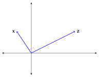
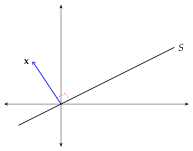
2.2.1Definition and Basic Properties¶

Let $\boldx$ and $\boldz$ be vectors in $\RR^N$ . If $\inner{\boldx, \boldz} = 0$ , then we write $\boldx \perp \boldz$ and call $\boldx$ and $\boldz$ orthogonal. In $\RR^2$ , $\boldx$ and $\boldz$ are orthogonal when they are perpendicular to one another, as in figure 2.12. For $\boldx \in \RR^N$ and $S \subset \RR^N$ , we say that $\boldx$ is orthogonal to $S$ if $\boldx \perp \boldz$ for all $\boldz \in S$ (figure 2.13), and we write $\boldx \perp S$ . A set of vectors $\{\boldz_1, \ldots, \boldz_K\} \subset \RR^N$ is called an orthogonal set if its elements are mutually orthogonal, that is, if $\boldz_j \perp \boldz_k$ whenever $j$ and $k$ are distinct.

Orthogonal sets and linear independence are closely related. For example,

While not every linearly independent set is orthogonal, an important partial converse to fact 2.2.2 is given in Section 2.2.4.

An orthogonal set $O \subset \RR^N$ is called an orthonormal set if $\| \boldu \| = 1$ for all $\boldu \in O$ . An orthonormal set that lies in and spans a linear subspace $S$ of $\RR^N$ is called an orthonormal basis of $S$ . It is, necessarily, a basis of $S$ . (Why?) The standard example of an orthonormal basis for all of $\RR^N$ is the canonical basis $\{\bolde_1, \ldots, \bolde_N\}$ .

By definition, if $O = \{\boldu_1, \ldots, \boldu_K\}$ is any basis of $S$ , then, for any $\boldx \in S$ , we can find unique scalars $\alpha_1, \ldots, \alpha_K$ such that $\boldx = \sum_{k=1}^K \alpha_k \boldu_k$ . While the values of these scalars are not always transparent, for an orthonormal basis they are easy to compute:

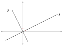
The proof is an exercise. Given $S \subset \RR^N$ , the orthogonal complement of $S$ is defined as

S^{\perp} := \setntn{\boldx \in \RR^N}{\boldx \perp S}

Figure 2.14 gives an example in $\RR^2$ .

Orthogonal complement of S — Figure 2.14:Orthogonal complement of $S$

Indeed, if $\boldx, \boldy \in S^{\perp}$ and $\alpha, \beta \in \RR$ , then $\alpha \boldx + \beta \boldy \in S^{\perp}$ because, for any $\boldz \in S$ ,

\inner{\alpha \boldx + \beta \boldy, \boldz} = \alpha \inner{ \boldx, \boldz} + \beta \inner{\boldy, \boldz} = \alpha \times 0 + \beta \times 0 = 0

2.2.2The Orthogonal Projection Theorem¶

A central problem in linear regression and many other applications is approximation of some $\boldy$ of $\RR^N$ by an element of a given subspace $S$ of $\RR^N$ . Stated more precisely, the problem is, given $\boldy$ and $S$ , to find the closest element $\hat \boldy$ of $S$ to $\boldy$ . Closeness is in terms of Euclidean norm, so $\hat \boldy$ is the minimizer of $\| \boldy - \boldz \|$ over all $\boldz \in S$ :

\hboldy = \argmin_{\boldz \in S} \|\boldy - \boldz\|

(2.9)

The next theorem tells us that a solution $\hboldy$ to this minimization problem always exists, as well as providing a means to identify it.

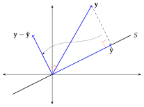
The intuition is easy to grasp from a graphical presentation. Figure 2.15 illustrates. Looking at the figure, we can see that the closest point to $\boldy$ in $S$ is the one point $\hboldy \in S$ such that $\boldy - \hboldy$ is orthogonal to $S$ .

For a full proof see, for example, theorem 5.16 of Çinlar & Vanderbei (2013). Let’s just cover sufficiency of the conditions in part (ii): Let $\boldy \in \RR^N$ and let $S$ be a linear subspace of $\RR^N$ . Let $\hat \boldy$ be a vector in $S$ satisfying $\boldy - \hat \boldy \perp S$ . Let $\boldz$ be any other point in $S$ . We have

\| \boldy - \boldz \|^2 = \| (\boldy - \hat \boldy) + (\hat \boldy - \boldz) \|^2 = \| \boldy - \hat \boldy \|^2 + \| \hat \boldy - \boldz \|^2

The second equality follows from $\boldy - \hat \boldy \perp S$ (why?) and the Pythagorian law. Since $\boldz$ was an arbitrary point in $S$ , we have $\| \boldy - \boldz \| \geq \| \boldy - \hat \boldy \|$ for all $\boldz \in S$ . Hence (2.9) holds.

Example 2.2.1

Let $\boldy \in \RR^N$ and let $\boldone \in \RR^N$ be the vector of ones. Let $S$ be the set of constant vectors in $\RR^N$ , meaning that all elements are equal. Evidently $S$ is the span of $\{\boldone\}$ . The orthogonal projection of $\boldy$ onto $S$ is $\hboldy := \bar y \boldone$ , where $\bar y := \frac{1}{N} \sum_{n=1}^N y_n$ . To see this, note that $\hboldy \in S$ clearly holds. Hence we only need to check that $\boldy - \hboldy$ is orthogonal to $S$ , for which it suffices to show that $\inner{\boldy - \hboldy, \boldone} = 0$ (see ex. 2.4.14). This is true because

\inner{\boldy - \hboldy, \boldone } = \inner{\boldy, \boldone} - \inner{\hboldy, \boldone} = \sum_{n=1}^N y_n - \bar y \inner{\boldone, \boldone} = 0

2.2.3Projection as a Mapping¶

In view of theorem 2.2.1, for each fixed linear subspace $S$ in $\RR^N$ , the operation

\boldy \; \mapsto \text{ the orthogonal projection of } \boldy \text{ onto } S

is a well-defined function from $\RR^N$ to $\RR^N$ . The function is typically denoted by $\boldP$ . For each $\boldy \in \RR^N$ , the symbol $\boldP \boldy$ represents the image of $\boldy$ under $\boldP$ , which is the orthogonal projection $\hboldy$ . $\boldP$ is called the orthogonal projection onto $S$ , and we write

\boldP = \proj S

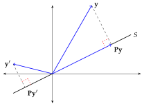
Figure 2.16 illustrates the action of $\boldP$ on two different vectors.

Orthogonal projection under \boldP — Figure 2.16:Orthogonal projection under $\boldP$

Using this notation, we can restate the orthogonal projection theorem, as well as adding some properties of $\boldP$ :

These results are not difficult to prove, given theorem 2.2.1. Linearity of $\boldP$ is left as an exercise (ex. 2.4.29). Parts (ii)–(iii) follow directly from theorem 2.2.1. To see (iv), observe that $\boldy$ can be decomposed as $\boldy = \boldP \boldy + \boldy - \boldP \boldy$ . Now apply the Pythagorean law. Part (v) follows from part (iv). Part (vi) follows from the definition of $\boldP \boldy$ as the closest point to $\boldy$ in $S$ . Part (vii) is an exercise.

Fact 2.2.6 is a fundamental result. It’s true because the right-hand side of (2.10) clearly lies in $S$ (being a linear combination of basis functions) and, for any $\boldu_j$ in the basis set

\inner{\boldy - \boldP \boldy, \boldu_j} = \inner{\boldy, \boldu_j } - \sum_{k=1}^K \inner{\boldy, \boldu_k} \inner{\boldu_k, \boldu_j} = \inner{\boldy, \boldu_j} - \inner{\boldy, \boldu_j } = 0

This is enough to confirm that $\boldy - \boldP \boldy \perp S$ (see ex. 2.4.14).

There’s one more essential property of $\boldP$ that we need to make note of: Suppose that we have two linear subspaces $S_1$ and $S_2$ of $\RR^N$ , where $S_1 \subset S_2$ . What then is the difference between (1) first projecting a point onto the bigger subspace $S_2$ , and then projecting the result onto the smaller subspace $S_1$ , and (2) projecting directly to the smaller subspace $S_1$ ? The answer is none—we get the same result:

2.2.4The Residual Projection¶

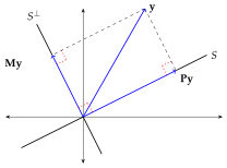
Consider the setting of the orthogonal projection theorem. Our interest is in projecting $\boldy$ onto $S$ , where $S$ is a linear subspace of $\RR^N$ . The closest point to $\boldy$ in $S$ is $\hboldy := \boldP \boldy$ where $\boldP = \proj S$ . Unless $\boldy$ was already in $S$ , some error $\boldy - \boldP \boldy$ remains. Tracking and managing this residual will be important to us, so let’s introduce an operator $\boldM$ that takes $\boldy \in \RR^N$ and returns the residual. We can define it as

\boldM := \boldI - \boldP

(2.11)

where $\boldI$ is the identity mapping on $\RR^N$ . For any $\boldy$ we have $\boldM \boldy = \boldI \boldy - \boldP \boldy = \boldy - \boldP \boldy$ as required. In regression analysis $\boldM$ shows up as a matrix called the “annihilator.” This is a pretty cool name, but it’s also not a great description of its function. In what follows we will refer to $\boldM$ as the residual projection.

Part (v) means that $\boldP \boldM \boldy = \boldM \boldP \boldy = \boldzero$ for all $\boldy \in \RR^N$ . Figure 2.17 illustrates the action of $\boldM$ . The results in fact 2.2.8 can be seen in the figure.

If $S_1$ and $S_2$ are two subspaces of $\RR^N$ with $S_1 \subset S_2$ , then $S_2^{\perp} \subset S_1^{\perp}$ . This means that the result in fact 2.2.7 is reversed for $\boldM$ .

As an application of the ideas above, let’s now discuss a procedure called Gram–Schmidt orthogonalization, which provides a fundamental link between the two major concepts discussed in this chapter: linear independence and orthogonality. It can be considered as a partial converse to fact 2.2.2.

The proof of theorem 2.2.3 provides an important algorithm for generating the orthonormal set $\{\boldu_1, \ldots, \boldu_K\}$ . The first step is to construct orthogonal sets $\{\boldv_1, \ldots, \boldv_k\}$ with span identical to $\{\boldb_1, \ldots, \boldb_k\}$ for each $k$ . The construction of $\{\boldv_1, \ldots, \boldv_K\}$ uses the so called Gram–Schmidt orthogonalization procedure. First, for each $k = 1, \ldots, K$ , let

$B_k := \Span\{\boldb_1, \ldots, \boldb_k\}$ ,
$\boldP_k := \proj B_k$ and $\boldM_k := \proj B_k^{\perp}$ ,
$\boldv_k := \boldM_{k-1} \boldb_k$ where $\boldM_0$ is the identity mapping, and
$V_k := \Span\{\boldv_1, \ldots, \boldv_k\}$ .

In step (iii) we map each successive element $\boldb_k$ into a subspace orthogonal to the subspace generated by $\boldb_1, \ldots, \boldb_{k-1}$ . In the exercises you are asked to show that $\{\boldv_1, \ldots, \boldv_K\}$ is an orthogonal set and $V_k = B_k$ for all $k$ (ex. 2.4.34). To complete the argument, we introduce the vectors $\boldu_k$ by $\boldu_k := \boldv_k / \| \boldv_k \|$ and confirm that this set of vectors $\{\boldu_1, \ldots, \boldu_k\}$ is orthonormal with span equal to $V_k$ . These results are also (solved) exercises.

2.3Further Reading¶

Good texts on vector spaces include Marcus & Minc (1988) and Jänich (1994).

2.4Exercises¶

In the next three exercises, the notation is as given in theorem 2.2.3 and the discussion immediately afterwards.

2.4.1Solutions to Selected Exercises¶

Solution to Exercise 2.4.8

There is an easy way to do this: We know that any linearly independent set of 3 vectors in $\RR^3$ will span $\RR^3$ . Since $\boldz \in \RR^3$ , this will include $\boldz$ . So all we need to do is show that the 3 vectors are linearly independent. To this end, take any scalars $\alpha_1, \alpha_2, \alpha_3$ with

\alpha_1 \begin{pmatrix} -4 \\ 0 \\ 0 \end{pmatrix} + \alpha_2 \begin{pmatrix} 0 \\ 2 \\ 0 \end{pmatrix} + \alpha_3 \begin{pmatrix} 0 \\ 0 \\ -1 \end{pmatrix} = \boldzero := \begin{pmatrix} 0 \\ 0 \\ 0 \end{pmatrix}

Written as three equations, this says that $-4 \alpha_1 = 0$ , $2 \alpha_2 = 0$ , and $-1 \alpha_3 = 0$ . Hence $\alpha_1 = \alpha_2 = \alpha_3 = 0$ , and therefore the set is linearly independent.

Solution to Exercise 2.4.15

We are asked to verify the equivalences in theorem 2.1.1 for the set $X := \{\boldx_1,\ldots, \boldx_K\}$ . We will prove the cycle (i) $\implies$ (ii) $\implies$ (iii) $\implies$ (i).

((i) $\implies$ (ii)) We aim to show that if (i) holds and $X_0$ is a proper subset of $X$ , then $\Span X_0$ is a proper subset of $\Span X$ . To simplify notation let’s take $X_0 := \{\boldx_2,\ldots, \boldx_K\}$ . Suppose, to the contrary, that $\Span X_0 = \Span X$ . Since $\boldx_1 \in \Span X$ , we must then have $\boldx_1 \in \Span X_0$ , from which we deduce the existence of scalars $\alpha_2, \ldots, \alpha_K$ such that $\boldzero = -\boldx_1 + \alpha_2 \boldx_2 + \cdots + \alpha_K \boldx_K$ . Since $-1 \neq 0$ , this contradicts part (i).

((ii) $\implies$ (iii)) The claim is that when (ii) holds, no vector in $X$ can be written as a linear combination of the others. Suppose, to the contrary, that $\boldx_1 = \alpha_2 \boldx_2 + \cdots + \alpha_K \boldx_K$ , say. Let $\boldy \in \Span X$ , so that $\boldy = \beta_1 \boldx_1 + \cdots + \beta_K \boldx_K$ . If we use the preceding equality to substitute out $\boldx_1$ , we get $\boldy$ as a linear combination of $\{\boldx_2, \ldots, \boldx_K\}$ alone. In other words, any element of $\Span X$ is in the span of the proper subset $\{\boldx_2, \ldots, \boldx_K\}$ . Contradiction.

((iii) $\implies$ (i)) The final claim is that $\alpha_1 = \cdots = \alpha_K = 0$ whenever $\alpha_1 \boldx_1 + \cdots + \alpha_K \boldx_K = \boldzero$ . Suppose, to the contrary, that there exist scalars with $\alpha_1 \boldx_1 + \cdots + \alpha_K \boldx_K = \boldzero$ and yet $\alpha_k \neq 0$ for at least one $k$ . It follows immediately that $\boldx_k = (1/\alpha_k) \sum_{j \neq k} \alpha_j \boldx_j$ . This contradicts (iii).

Solution to Exercise 2.4.16

The aim is to prove fact 2.1.4. Regarding the part (i), let’s take $X$ as linearly independent and show that the subset $X_0 := \{\boldx_1,\ldots, \boldx_{K-1}\}$ is linearly independent. (The argument for more general subsets is similar.) Suppose, to the contrary, that $X_0$ is linearly dependent. Then, by the definition, we can take $\alpha_1, \ldots, \alpha_{K-1}$ not all zero with $\sum_{k=1}^{K-1} \alpha_k \boldx_k = \boldzero$ . Letting $\alpha_K =0$ , we can write this as $\sum_{k=1}^K \alpha_k \boldx_k = \boldzero$ . Since not all coefficients are zero, we have contradicted linear independence of $X$ .

Regarding (ii), let $X := \{\boldx_1,\ldots, \boldx_K\}$ be linearly independent and suppose that $\boldx_j = \boldzero$ . Then by setting $\alpha_k = 0$ for $k\neq j$ and $\alpha_j = 1$ , we can form scalars not all equal to zero with $\sum_{k=1}^K \alpha_k \boldx_k = \boldzero$ .

Regarding (iii), let $X := \{\boldx_1,\ldots, \boldx_K\} \subset \RR^N$ be linearly independent and let $\boldx_{K+1}$ be any point in $\RR^N$ such that $\boldx_{K+1} \notin \Span X$ . The claim is that $X \cup \{\boldx_{K+1}\}$ is linearly independent. Suppose, to the contrary, that there exist $\alpha_1, \ldots, \alpha_K, \alpha_{K+1}$ not all zero such that $\sum_{k=1}^{K+1} \alpha_k \boldx_k = \boldzero$ . There are two possibilities for $\alpha_{K+1}$ , both of which lead to a contradiction: First, if $\alpha_{K+1} = 0$ , then, since $\alpha_1, \ldots, \alpha_K, \alpha_{K+1}$ are not all zero, at least one of $\alpha_1, \ldots, \alpha_K$ are nonzero, and moreover $\sum_{k=1}^K \alpha_k \boldx_k = \sum_{k=1}^{K+1} \alpha_k \boldx_k = \boldzero$ . This contradicts our assumption of independence on $X$ . Second, if $\alpha_{K+1} \neq 0$ , then from $\sum_{k=1}^{K+1} \alpha_k \boldx_k = \boldzero$ we can express $\boldx_{K+1}$ as a linear combination of elements of $X$ . This contradicts the hypothesis that $\boldx_{K+1} \notin \Span X$ .

Solution to Exercise 2.4.18

The aim is to prove fact 2.1.6. Suppose that $S$ and $S'$ are $K$ -dimensional linear subspaces of $\RR^N$ with $S \subset S'$ . We claim that $S = S'$ . To see this, observe that by the definition of dimension, $S$ is equal to $\Span B$ where $B$ is a set of $K$ linearly independent basis vectors $\{\boldb_1, \ldots, \boldb_K\}$ . If $S \neq S'$ , then there exists a vector $\boldx \in S'$ such that $\boldx \notin \Span B$ . In view of theorem 2.1.1, the set $\{\boldx, \boldb_1, \ldots, \boldb_K\}$ is linearly independent. Moreover, since $\boldx \in S'$ and since $B \subset S \subset S'$ , we now have $K+1$ linearly independent vectors inside $S'$ . At the same time, being $K$ -dimensional, we know that $S'$ is spanned by $K$ vectors. This contradicts theorem 2.1.3.

Regarding part (ii), suppose that $S$ is an $M$ -dimensional linear subspace of $\RR^N$ where $M < N$ and yet $S = \RR^N$ . Then we have a space $S$ spanned by $M < N$ vectors that also contains the $N$ linearly independent canonical basis vectors. We are led to another contradiction of theorem 2.1.3. Hence $S = \RR^N$ cannot hold.

Solution to Exercise 2.4.19

Regarding part (i), let $B$ be a basis of $\Span X$ . By definition, $B$ is a linearly independent subset of $\Span X$ . Since $\Span X$ is spanned by $K$ vectors, theorem 2.1.3 implies that $B$ has no more than $K$ elements. Hence, $\dim \Span X \leq K$ .

Regarding part (ii), suppose first that $X$ is linearly independent. Then $X$ is a basis for $\Span X$ . Since $X$ has $K$ elements, we conclude that $\dim \Span X = K$ . Conversely, if $\dim \Span X = K$ , then $X$ must be linearly independent. If $X$ were not linearly independent, then there would exist a proper subset $X_0$ of $X$ such that $\Span X_0 = \Span X$ . By part (i) of this theorem, we then have $\dim \Span X_0 \leq \# X_0 \leq K - 1$ . Therefore $\dim \Span X \leq K - 1$ , a contradiction.

Solution to Exercise 2.4.20

Let $T \colon \RR^N \to \RR^N$ be nonsingular, and let $T^{-1}$ be its inverse. To see that $T^{-1}$ is linear, we need to show that for any pair $\boldx, \boldy$ in $\RR^N$ (which is the domain of $T^{-1}$ ) and any scalars $\alpha$ and $\beta$ , the following equality holds:

T^{-1}(\alpha \boldx + \beta \boldy) = \alpha T^{-1}\boldx + \beta T^{-1} \boldy

(2.12)

In the proof we will exploit the fact that $T$ is by assumption a linear bijection.

Pick any vectors $\boldx, \boldy \in \RR^N$ and any two scalars $\alpha, \beta$ . Since $T$ is a bijection, we know that $\boldx$ and $\boldy$ have unique preimages under $T$ . In particular, there exist unique vectors $\boldu$ and $\boldv$ such that $T\boldu = \boldx$ and $T\boldv = \boldy$ . Using these definitions, linearity of $T$ and the fact that $T^{-1}$ is the inverse of $T$ , we have

T^{-1}(\alpha \boldx + \beta \boldy) = T^{-1}(\alpha T\boldu + \beta T \boldv) = T^{-1}(T(\alpha \boldu + \beta \boldv)) = \alpha \boldu + \beta \boldv = \alpha T^{-1} \boldx + \beta T^{-1} \boldy

This chain of equalities confirms (2.12).

Solution to Exercise 2.4.21

A collection of equivalent statements such as this is usually proved via a cycle of implications, with the form (i) $\implies$ (ii) $\implies \cdots \implies$ (vi) $\implies$ (i). However, in this case the logic is clearer if we directly show that all statements are equivalent to linear independence of $V$ .

First observe equivalence of the onto property and linear independence of $V$ via

T \text{ onto } \; \iff \; \range T = \RR^N \; \iff \; \Span V = \RR^N

by fact 2.1.7. The last statement is equivalent to linear independence of $V$ by theorem 2.1.4.

Next let’s show that $\kernel T = \{ \boldzero \}$ implies linear independence of $V$ . To this end, suppose that $\kernel T = \{ \boldzero \}$ and let $\alpha_1, \ldots, \alpha_N$ be such that $\sum_{n=1}^N \alpha_n T\bolde_n = \boldzero$ . By linearity of $T$ , we then have $T(\sum_{n=1}^N \alpha_n \bolde_n) = \boldzero$ . Since $\kernel T = \{ \boldzero \}$ , this means that $\sum_{n=1}^N \alpha_n \bolde_n = \boldzero$ , which in view of independence of $\{\bolde_1, \ldots, \bolde_N\}$ , implies $\alpha_1 = \cdots = \alpha_N = 0$ . This establishes that $V$ is linearly independent.

Now let’s check that linear independence of $V$ implies $\kernel T = \{ \boldzero \}$ . To this end, let $\boldx$ be a vector in $\RR^N$ such that $T\boldx = \boldzero$ . We can represent $\boldx$ in the form $\sum_{n=1}^N \alpha_n \bolde_n$ for suitable scalars $\{\alpha_n\}$ . From linearity and $T\boldx = \boldzero$ , we get $\sum_{n=1}^N \alpha_n T\bolde_n = \boldzero$ . By linear independence of $V$ , this implies that each $\alpha_n = 0$ , whence $\boldx = \boldzero$ . Thus $\kernel T = \{ \boldzero \}$ as claimed.

From fact 2.1.8 we have $\kernel T = \{ \boldzero \}$ iff $T$ is one-to-one, so we can now state the following equivalences

T \text{ onto } \iff V \text{ linearly independent } \iff T \text{ one-to-one }

(2.13)

If $T$ is a bijection, then $T$ is onto and hence $V$ is linearly independent by (2.13). Conversely, if $V$ is linearly independent then $T$ is both onto and one-to-one by (2.13). Hence $T$ is a bijection.

Finally, equivalence of linear independence of $V$ and the statement that $V$ forms a basis of $\RR^N$ is immediate from the definition of bases and theorem 2.1.4.

Solution to Exercise 2.4.22

Regarding part (i), let $K < N$ and let $T \colon \RR^K \to \RR^N$ be linear. $T$ cannot be onto because, if $T$ were onto, then we would have $\range T = \RR^N$ , in which case the vectors in $V = \{T\bolde_1, \ldots, T\bolde_K\}$ in fact 2.1.7 would span $\RR^N$ , despite having only $K < N$ elements. This is impossible. (Why?)

Regarding part (ii), let $T \colon \RR^K \to \RR^N$ be linear and let $K > N$ . Seeking a contradiction, suppose in addition that $T$ is one-to-one. Let $\{\alpha_k\}_{k=1}^K$ be such that $\sum_{k=1}^K \alpha_k T \bolde_k = \boldzero$ . By linearity, $T(\sum_{k=1}^K \alpha_k \bolde_k) = \boldzero$ , and since $T$ is one-to-one and $T \boldzero = \boldzero$ , this in turn implies $\sum_{k=1}^K \alpha_k \bolde_k = \boldzero$ . Since the canonical basis vectors are linearly independent, it must be that $\alpha_1 = \cdots = \alpha_K = 0$ . From this we conclude that $\{T \bolde_1, \ldots, T\bolde_K\}$ is linearly independent. Thus $\RR^N$ contains $K$ linearly independent vectors, despite the fact that $N < K$ . This is impossible by theorem 2.1.3.

Solution to Exercise 2.4.29

Fix $\alpha, \beta \in \RR$ and $\boldx, \boldy \in \RR^N$ . The claim is that

\boldP (\alpha \boldx + \beta \boldy) = \alpha \boldP \boldx + \beta \boldP \boldy

To verify this equality, we need to show that the right-hand side is the orthogonal projection of $\alpha \boldx + \beta \boldy$ onto $S$ . Going back to theorem 2.2.1, we need to show that (i) $\alpha \boldP \boldx + \beta \boldP \boldy \in S$ and (ii) for any $\boldz \in S$ , we have

\inner{\alpha \boldx + \beta \boldy - (\alpha \boldP \boldx + \beta \boldP \boldy), \boldz} = 0

Here (i) is immediate, because $\boldP \boldx$ and $\boldP \boldy$ are in $S$ by definition, and, moreover $S$ is a linear subspace. To see that (ii) holds, just note that

\inner{\alpha \boldx + \beta \boldy - (\alpha \boldP \boldx + \beta \boldP \boldy), \boldz } = \alpha \inner{\boldx - \boldP \boldx, \boldz} + \beta \inner{\boldy - \boldP \boldy, \boldz}

By definition, the projections of $\boldx$ and $\boldy$ are orthogonal to $S$ , so we have $\inner{\boldx - \boldP \boldx, \boldz} = \inner{\boldy - \boldP \boldy, \boldz} = 0$ . We are done.

Solution to Exercise 2.4.32

From the triangle inequality we have

\| \boldx \| = \| \boldx - \boldy + \boldy \| \leq \| \boldx - \boldy \| + \| \boldy \|

- \| \boldx - \boldy \| \leq \| \boldx \| - \| \boldy \| \leq \| \boldx - \boldy \|

This is equivalent to $| \| \boldx \| - \| \boldy \| | \leq \| \boldx - \boldy \|$ .

Solution to Exercise 2.4.34

To see that $V_k = B_k$ for all $k$ , fix $k$ and consider the claim that $V_k \subset B_k$ . By definition, $\boldv_k = \boldb_k - \boldP_{k-1} \boldb_k$ , and the two terms on the right-hand side lie in $B_k$ . Hence $\boldv_k \in B_k$ . Since spans increase as we add more elements, it follows that $\boldv_j \in B_k$ for $j \leq k$ . In other words, $\{\boldv_1, \ldots, \boldv_k\} \subset B_k$ . Since $B_k$ is a linear subspace, we have $V_k \subset B_k$ .

An induction argument shows that $B_k \subset V_k$ also holds. Clearly it holds for $k=1$ . Suppose that it also holds for $k-1$ . From the definition of $\boldv_k$ , we have $\boldb_k = \boldP_{k-1} \boldb_k + \boldv_k$ . The first term on the right-hand side lies in $B_{k-1}$ , which, by our induction hypothesis, satisfies $B_{k-1} \subset V_{k-1} \subset V_k$ . The second term on the right-hand side is $\boldv_k$ , which obviously lies in $V_k$ . Hence both terms are in $V_k$ , and therefore $\boldb_k \in V_k$ . Using arguments analogous to the end of the last paragraph leads us to $B_k \subset V_k$ .

Solution to Exercise 2.4.36

Since $\{\boldv_1, \ldots, \boldv_k\}$ is orthogonal, the family $\{\boldu_1, \ldots, \boldu_k\}$ will be orthonormal provided that the norm of each element is 1. This is true by construction, since $\boldu_k := \boldv_k / \| \boldv_k \|$ . The only concern is that $\| \boldv_k \| = 0$ might hold for some $k$ . But $\boldv_k = \boldzero$ is impossible because, if it was to hold, then by (vii) of theorem 2.2.2 we would have $\boldb_k \in B_{k-1}$ , contradicting linear independence of $\{\boldb_1, \ldots, \boldb_K\}$ .

The proof that $\Span\{\boldu_1, \ldots, \boldu_k\} = V_k$ is straightforward and left for you.

Footnotes¶

In some instances, the notion of scalar multiplication includes multiplication of vectors by complex numbers. In what follows we will work almost entirely with real scalars. Hence scalar multiplication means real scalar multiplication unless otherwise stated.
↩
$A$ is a proper subset of $B$ if $A \subset B$ and $A \neq B$ .
↩
Hint: There’s no need to go taking derivatives and setting them equal to zero. An easier proof exists. If you’re stuck, consider the Cauchy–Schwarz inequality.
↩
Hint: Use the triangle inequality.
↩

References¶

Jänich, K. (1994). Linear Algebra. New York: Springer.
Çinlar, E., & Vanderbei, R. J. (2013). Real and Convex Analysis. New York: Springer.
Marcus, M., & Minc, H. (1988). Introduction to Linear Algebra. Mineola, NY: Dover Publications.