National Graduate Institute for Policy Studies (GRIPS)
The previous chapter was relatively abstract but it sets us up nicely to study the kinds of practical problems from linear algebra that we encounter in statistics and econometrics. This chapter treats many of the core problems in linear algebra, frequently relating them back to our analysis of vectors and linear maps in chapter 2.
The symbol ank stands for the element in the nth row of the kth column. Often these elements represent coefficients in a system of linear equations, such as
For obvious reasons, A is also called a vector if either N=1 or K=1. In the former case, A is called a row vector, while in the latter case it is called a column vector. When convenient, we will use the notation rownA to refer to the nth row of A, and colkA to refer to its kth column.
We extend the notation 0 and 1 from vectors to matrices, in the sense that these symbols will also represent matrices with all elements equal to zero and one respectively. Dimensions will be stated explicitly or clear from context.
If A is N×K and N=K, then A is called square. For an N×N matrix A, the N elements of the form ann for n=1,…,N are called the principal diagonal:
a11a21⋮aN1a12a22⋮aN2⋯⋯⋯a1Na2N⋮aNN
The unique N×N matrix with ones on the principle diagonal and zeros elsewhere is called the identity matrix, and denoted by I:
I:=10⋮001⋮0⋯⋯⋯00⋮1
Note that colnI=en, the nth canonical basis vector in RN.
Just as was the case for vectors, a number of algebraic operations are defined for matrices. The first two, scalar multiplication and addition, are immediate generalizations of the vector case: For γ∈R, we let
Addition is only defined for matrices that have identical shape.
The matrix productC=AB of matrices A and B is formed by taking as its i,jth element the inner product of the ith row of A and the jth column of B. That is,
Since inner products are only defined for vectors of equal length, we need the length of the rows of A to be equal to the length of the columns of B. In other words, if A is N×K and B is J×M, then we require K=J. The resulting matrix AB is N×M. Here’s the rule to remember:
A is N×K and B is K×M⟹AB is N×M
Matrix multiplication is not commutative: AB and BA are not in general equal. In most other ways it behaves like ordinary multiplication:
Here and below we use the word conformable to indicate dimensions are such that the operation in question makes sense. For example, two matrices are conformable for addition if they have the same number of rows and columns.
The kth power of a square matrix A is defined as
Ak:=k termsA⋯A
If B is such that B2=A, then B is called the square root of A and written A.
Before going further, let’s state the fundamental connection between matrix multiplication and the more elementary notion of linear combinations of vectors, as introduced in Section 2.1.2: Given N×K matrix A and K×1 column vector x, the product Ax is an N×1 column vector formed as a linear combination of the columns of A, with scalars x1,…,xK. In symbols,
One of the most useful ways to think about matrices is as maps from one vector space to another. In particular, an N×K matrix A can be thought of as a map sending a vector x∈RK into a new vector y=Ax in RN. As the next theorem shows, these maps are always linear. In fact, they are the only linear functions. In other words, the set of linear functions from RK to RN and the set of N×K matrices are in one-to-one correspondence:
When we consider the problem of solving a system of linear equations such as Ax=b, the first issue we need to concern ourselves with is existence. Can we find an x that satisfies this equation, for any given b? A bit of thought will convince you that this is the same question as: Is the corresponding linear map Tx=Ax an onto function? (See Section 15.2 for the definition.) Equivalently, is rngT equal to all of RN?
The range of T is all vectors of the form Tx=Ax where x varies over RK. We just saw in Section 3.1.1 that, for any x∈RK, we have Ax=∑k=1KxkcolkA. It follows that rngT is equal to the column space of A, which is by definition the span of the columns of A. We represent it by the symbol
How large is the column space of a given matrix? To answer that question, we have to say what "large" means. In the context of linear algebra, size of subspaces is usually measured by dimension. The dimension of colspaceA is known as the rank of A. That is,
rankA:=dimcolspaceA
A is said to have full column rank if rankA is equal to K, the number of its columns. The reason we say “full” rank here is that, by definition, colspaceA is the span of K vectors. Hence, by part (i) of theorem 2.1.6, we must have dimcolspaceA⩽K. In other words, the rank of A is less than or equal to K. A is said to have full column rank when this maximum is achieved.
When is this maximum achieved? By part (ii) of theorem 2.1.6, this will be the case precisely when the columns of A are linearly independent. Let’s state this as a fact:
Perhaps the most common problem in linear algebra is solving systems of linear equations. A generic representation is Ax=b, where x contains the unknowns and A and b are given. There are a variety of scenarios depending on the properties of A. For now let’s consider the case where A is N×N, and seek conditions on A under which, for every b∈RN, there exists exactly one x∈RN such that Ax=b.
The best way to understand this problem is as follows. Let T be the linear map Tx=Ax. The question we are asking here is: When does each point b∈RN have one and only one preimage under T? In other words, when is T a bijection?
To answer this question, we can refer back to the discussion in Section 2.1.7. We saw there that linear bijections are called nonsingular functions, and we discussed a number of equivalences for this property. The next fact replicates these equivalences in the language of matrices.
These results can all be verified using theorem 2.1.7 by checking the corresponding implications for Tx=Ax. For example, it’s easy to see that if en is the nth canonical basis vector of RN, then
Ten=Aen=colnA
and hence the condition of linear independence of {Te1,…,TeN} in theorem 2.1.7 translates to linear independence of the columns of A.
Following common usage, if any of the equivalent conditions in fact 3.1.3 are true we will call not just the map T but also the underlying matrix Anonsingular. If any one—and hence all—of these conditions fail, then A is called singular.
Any bijection has an inverse (see Section 15.2). In fact any nonsingular map T has a nonsingular inverse T−1 (see fact 2.1.9). In the present setting, where T is generated by a matrix A, the inverse T−1 is also associated with a matrix, called the inverse of A. The next theorem gives details:
For this reason, nonsingular matrices are also referred to as invertible. The proof of theorem 3.1.2 is a solved exercise (ex. 3.5.5).
As stated in the next fact, to show that A is invertible and B is the inverse of A, it suffices to show that B is either a left inverse, in the sense that BA=I, or a right inverse, in the sense that AB=I. A proof is given in Section 3.1.4.
The next fact collects more useful results about inverse matrices.
The relation (AB)−1=B−1A−1 is just a special case of the analogous rule for inversion of bijections (see fact 15.2.1). But you can also prove the equality directly by confirming that B−1A−1 is a right inverse (or left inverse) of AB.
To each square matrix A, we can associate a unique number detA called the determinant of A. To define it, let S(N) be the set of all bijections from {1,…,N} to itself. For π∈S(N) we define the signature of π as
sgn(π):=m<n∏m−nπ(m)−π(n)
The determinant of N×N matrix A is then given as
detA:=π∈S(N)∑sgn(π)n=1∏Naπ(n)n
We won’t concern ourselves with the details of this definition. For now it’s enough to know the following facts:
In the 2×2 case one can show that the determinant satisfies
As an example of how these results can be useful, let’s go back and prove fact 3.1.4. Fix square matrix A and suppose that a right inverse B exists, in the sense that AB=I. This equality implies that both A and B are nonsingular, since applying det to both sides of AB=I and using the rules in fact 3.1.6 gives det(A)det(B)=1. It follows that both detA and detB are nonzero. Hence both matrices are nonsingular.
To show that B is the inverse of A, we just need to check that, in addition to AB=I, we have BA=I. To obtain the latter equality from the former, premultiply the former by B to get BAB=B and then postmultiply by B−1 to get BA=I. The proof for the left inverse case is similar.
lower triangular if each element strictly above the principal diagonal is zero,
upper triangular if every element strictly below the principal diagonal is zero, and
triangular if it is either upper or lower triangular.
For example, if we define
L:=123056001andU:=100250361
then L and U are lower and upper triangular respectively. The great advantage of triangular matrices is that the associated linear equations are simple to solve using either forward or backward substitution. For example, with the system
the top equation involves only x1, so we can solve for its value directly. Plugging this value into the second equation, we can solve for x2 and so on.
An even better situation arises when our matrix is both upper and lower triangular. These are the diagonal matrices. In other words, a square matrix A is diagonal if all entries off the principal diagonal are zero. For example, the identity matrix is diagonal.
The following notation is often used to define diagonal matrices:
diag(d1,…,dN):=d10⋮00d2⋮0⋯⋯⋯00⋮dN
With diagonal matrices it is trivial to compute powers, roots, inverses and products:
You can check parts (i) and (ii) directly. The other claims follow from (i) and (ii).
A square matrix A is called symmetric if A⊺=A, or, equivalently, ank=akn for every k and n. Note that A⊺A and AA⊺ are always well-defined and symmetric.
Note that if a and b are N×1 vectors, then the matrix product a⊺b=b⊺a is equal to ∑n=1Nanbn, which is the same as the inner product ⟨a,b⟩. In what follows we’ll often work with column vectors and use matrix product rather than inner product notation.
Let A be N×N. As in Section 3.1.2, think of A as a linear map, so that Ax is the image of x under A. In general, A will map x to some arbitrary new location but sometimes x will only be scaled. That is,
for some scalar λ. If x and λ satisfy (3.6) and x is nonzero, then x is called an eigenvector of A, λ is called an eigenvalue, and (x,λ) is called an eigenpair.
Consider now the matrix
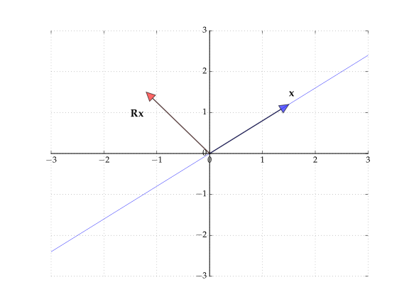
R:=(01−10)
that rotates any point counterclockwise by 90∘, as shown in figure 3.1. This rotation causes the scaling in (3.6) to fail for any λ∈R and nonzero x∈R2. If, however, we admit the possibility that λ and the elements of x can be complex, then (3.6) can hold. For example, direct calculation confirms that λ=i and x=(1,−i)⊺ is an eigenpair for R. It turns out that contemplation of complex eigenpairs is useful. Here eigenpairs are taken to be complex-valued unless explicitly stated to be real.
Here I is the N×N identity. Exercise 3.5.17 asks you to confirm this important fact. For the 2×2 matrix in (3.4), the rule for the 2×2 determinant in (3.4), fact 3.2.6 and a little bit of algebra imply that its eigenvalues are given by the two roots of the polynomial expression
λ2−(a+d)λ+(ad−bc)=0
More generally, given any N×N matrix A, it can be shown via the fundamental theorem of algebra that there exist complex numbers λ1,…,λN, not necessarily distinct, such that
It is clear that each λn satisfies det(A−λnI)=0 and hence is an eigenvalue of A. In particular, λ1,…,λN is the set of eigenvalues of A, although it’s worth repeating that these numbers are not necessarily distinct.
It is immediate from (i) that A is nonsingular ⟺ all its eigenvalues are nonzero.
In statistics and econometrics we often encounter quadratic expressions. In general, given symmetric N×N matrix A, the quadratic function or quadratic form on RN associated with A is the map Q defined by
Q(x):=x⊺Ax=j=1∑Ni=1∑Naijxixj
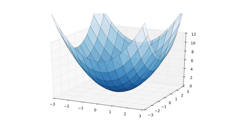
To give a simple illustration, let N=2 and let A be the identity matrix I. In this case,
Q(x)=∥x∥2=x12+x22
A 3D graph of this function is shown in figure 3.2.
One thing you’ll notice about this function is that its graph lies everywhere above zero, or Q(x)⩾0. In fact we know that ∥x∥2 is nonnegative and will be zero only when x=0. Hence the graph touches zero only at the point x=0. Many other choices of A yield a quadratic form with this property. Such A are said to be positive definite. More generally, an N×N symmetric matrix A is called
nonnegative definite if x⊺Ax⩾0 for all x∈RN,
positive definite if x⊺Ax>0 for all x∈RN with x=0,
nonpositive definite if x⊺Ax⩽0 for all x∈RN, and
negative definite if x⊺Ax<0 for all x∈RN with x=0.
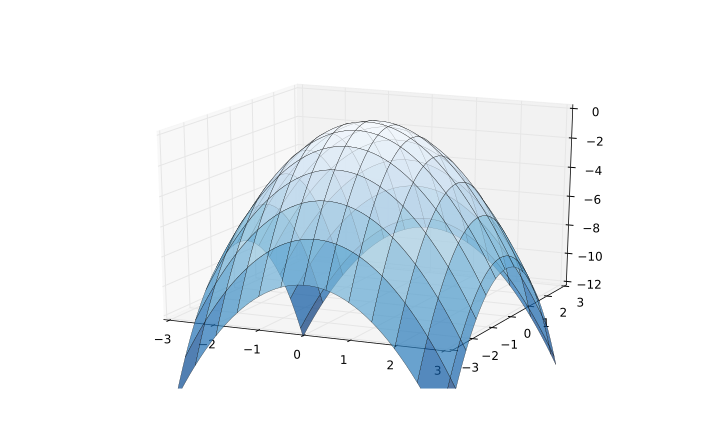
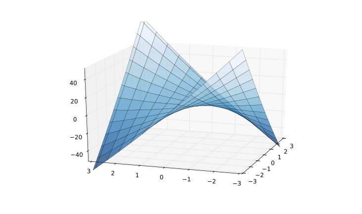
If A fits none of these categories, then A is called indefinite. Figure 3.3 shows the graph of a negative definite quadratic function. Now the function is hill-shaped, and 0 is the unique global maximum. Figure 3.4 shows an indefinite form.
Figure 3.4:Quadratic function Q(x)=x12/2+8x1x2+x22/2
The easiest case for detecting definiteness is when the matrix A is diagonal, since
A=diag(d1,…,dN)impliesQ(x)=d1x12+⋯+dNxN2
From the right-hand expression we see that a diagonal matrix is positive definite if and only if all diagonal elements are positive. Analogous statements are true for nonnegative, nonpositive and negative definite matrices. The next fact generalizes this idea and is proved in Section 3.3.4.
This section collects some essential results on projection and decomposition of matrices. The projection material takes our abstract projection theory from Section 2.2 and translates it into the more concrete language of matrices.
As stated in theorem 2.2.2, given any subspace S, the corresponding projection P=projS is a linear map from RN to RN. In view of theorem 3.1.1, it follows that there exists an N×N matrix P^ such that Px=P^x for all x∈RN. In fact we’ve anticipated this in the notation P, and from now on P will also represent the corresponding matrix. But what does this matrix look like?
This result generalizes fact 2.2.6, which pertains to projection onto the span of an orthonormal basis. The expression in (3.8) is more complex, but at the same time it applies to any basis, orthonormal or otherwise. We further explore the connection between the two results in Section 3.3.3. For the proof of theorem 3.3.1 see exercise 3.5.30 and its solution.
The construction of P in (3.8) implicitly assumes that B⊺B is nonsingular. This is justified because B has full column rank (see ex. 3.5.28). As usual, we let M=I−P denote the residual projection.
Idempotence of P and M can be checked by direct calculation. A better understanding is obtained by reflecting on the fact that projecting onto a subspace twice is the same as projecting once. After one projection the vector is already in the subspace. See fact 2.2.8.
For orthogonal projections, we can say more:
To see why rankP=dimS, recall that the rank of a linear map is the dimension of its range. When P=projS, the range of P is exactly S.
To show that traceP=dimS also holds, we can appeal to fact 3.3.3. There’s also a nice direct proof. See exercise 3.5.27 and its solution. Once we know that traceP=dimS, it’s clear that traceM=N−dimS because
In Section 3.1.3 we talked about solving equations of the form Ax=b when A is square. In statistics and econometrics, we often work the case where A is N×K and K⩽N. When the inequality is strict, the system of equations is said to be overdetermined.
Consider the problem of whether or not there exists a vector x satisfying Ax=b in this setting. Intuitively, when the number of equations is larger than the number of unknowns (N>K) we may not be able to find an x that satisfies all N equations. There are several equivalent ways to formalize this intuition. The linear map T:RK→RN corresponding to A is Tx=Ax (see Section 3.1.2). We know the following statements to be equivalent:
there exists an x∈RK with Ax=b.
b∈colspaceA.
b∈rngT.
We also know from theorem 2.1.8 that when K<N, the function T cannot be onto, and hence it’s possible that b lies outside the range of T.
In fact we can say more than this. When K<N, the scenario b∈colspaceA is in some sense very rare. The reason is that the dimension of colspaceA, which is precisely the rank of A, is less than or equal to K (see Section 3.1.2) and hence strictly less than N. There is a sense in which K-dimensional subspaces of RN are negligible, and hence the “chance” of b happening to lie in this subspace is tiny.[1]
As a result the standard approach is to admit that an exact solution may not exist, and to focus instead on finding a x∈RK such that Ax is as close to b as possible. It’s natural that "close to" is defined in terms of ordinary Euclidean norm, which leads us to the minimization problem
This is called a least squares problem because solving (3.11) is the same as minimizing ∥b−Ax∥2 with respect to x, and the squared norm is, by definition, a sum of squares. Assuming as before that A is N×K with K⩽N and b is N×1, we can use the orthogonal projection theorem to solve (3.11) as follows:
In the expression for x^ in (3.12), the matrix (A⊺A)−1A⊺ is called the pseudoinverse of A. If K=N—that is, if A is in fact square—then, under our full rank assumption, the pseudoinverse reduces to the inverse A−1, and the least squares solution x^ in (3.12) reduces to the expression given in (3.3).
What happens if we drop the assumption that the columns of A are linearly independent? The set colspaceA is still a linear subspace, and the orthogonal projection theorem still gives us a closest point Pb to b in colspaceA. Since Pb∈colspaceA, there still exists a vector x^ such that Pb=Ax^. The problem is that now there exists an infinity of such vectors. Exercise 3.5.34 asks you to prove this.
The QR decomposition of a given matrix A is a product of the form QR, where the first matrix has orthonormal columns and the second is upper triangular. This factorization has many applications, including least squares problems and the computation of eigenvalues. The decomposition is based on Gram–Schmidt orthogonalization.
Given the decomposition A=QR, the least squares solution x^ defined in (3.12) can also be written as x^=R−1Q⊺b (ex. 3.5.32). Premultiplying by R converts this expression to Rx^=Q⊺b, which is easy to solve because R is triangular (see Section 3.2.1).
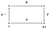
One important concept in dynamic systems and related fields is topological conjugacy. If f:A→A and g:B→B, then g is said to be topologically conjugate to f whenever there exists a continuous bijection τ:B→A such that f=τ∘g∘τ−1. The idea is that the action of f can be replicated by transporting a point into the domain of g, applying g, and then transporting it back. This can be beneficial if g is somehow simpler than f.
In the case of linear maps—that is, matrices—it is natural to study conjugacy in a setting where the bijection is also required to be linear. In linear algebra this is called similarity. In particular, a square matrix A is said to be similar to another matrix B if there exists an invertible matrix P such that A=PBP−1. Figure 3.5 shows the conjugate relationship of the two matrices when thought of as maps.
As discussed above, similarity of A to a given matrix B is most useful when B is somehow simpler than A, or more amenable to a given operation. The simplest kind of matrices we work with are diagonal matrices, so similarity to a diagonal matrix is particularly desirable. If A is similar to a diagonal matrix, then A is called diagonalizable.
If A=PΛP−1 where Λ is diagonal, it follows immediately that the elements on the principal diagonal of Λ are the eigenvalues of A, and that the columns of P are eigenvectors. To see this, observe that A=PΛP−1 implies AP=PΛ. Equating the nth column on each side gives Apn=λnpn, where pn:=colnP. Finally, pn is not the zero vector because otherwise P would not be invertible. Let’s summarize:
But when is A diagonalizable? The only thing we need to make the expression A=PΛP−1 work is for P to be invertible. This explains the next fact.
If A does have N linearly independent eigenvectors, then we are in good shape—diagonalization is possible. But can we do any better? The matrix Λ cannot really be simplified, but in some cases P can be. In particular, things are even nicer if P has orthonormal columns—that is, its columns form an orthonormal set, and hence an orthonormal basis of RN. These kinds of matrices are called orthogonal matrices. Here are some nice properties of such matrices.
The first result tells us is that if A=QΛQ−1 and Q has orthonormal columns, then A=QΛQ⊺. It’s easy to see from this expression that A must be symmetric, so if we hope to diagonalize with this extra orthonormal property, then we shouldn’t look beyond symmetric matrices. The following fundamental theorem tells us that this form of diagonalization is possible precisely when A is symmetric.
This is one version of the spectral decomposition theorem. See, for example, §10.3 of Jänich (1994). QΛQ⊺ is called the symmetric eigenvalue decomposition of A. It’s not hard to see that its action on a given N×1 vector x can be written as
Ax=n=1∑Nλn(un⊺x)un
where λn is the nth eigenvalue of A and un=colnQ. Compare with x=∑n=1N(un⊺x)un, which is true by fact 2.2.3.
One nice application of the spectral theorem is a proof of fact 3.2.8, which states among other things that symmetric matrix A is positive definite if and only if its eigenvalues are all positive. Exercise 3.5.23 and its solution step you through the arguments.
Here QΛQ⊺ is the spectral decomposition of A. To check that QΛQ⊺ is a square root just multiply. Λ exists because A is nonnegative definite, and hence its eigenvalues are nonnegative (see fact 3.2.8 and fact 3.2.2).
By combining our results on spectral decomposition with the QR decomposition discussed in Section 3.3.3, we can prove the following well-known fact:
This decomposition is called the Cholesky decomposition. The proof is obtained by writing
A=QΛQ⊺=QΛΛQ⊺=(ΛQ⊺)⊺ΛQ⊺
and applying the QR decomposition to ΛQ⊺. This allows us to write ΛQ⊺=Q~R, where R is nonsingular and upper triangular, and Q~ has orthonormal columns. Because the columns of Q~ are orthonormal,
A=(Q~R)⊺Q~R=R⊺Q~⊺Q~R=R⊺R
Our decomposition has the properties stated in fact 3.3.10.
Given vector sequence {xn} in RK and any point x∈RK, we say that {xn}converges to x and write xn→x if, for any ϵ>0, there exists an N∈N such that ∥xn−x∥<ϵ whenever n⩾N. Another way to say this is that the real-valued sequence zn:=∥xn−x∥ converges to zero in R as n→∞.
For econometrics it is helpful if we extend the notion of convergence to matrices. We can do this in a parallel fashion by defining norms over matrices. The matrix norm of N×K matrix A is defined as
In this expression there are two different norms in play: The left-hand side is a matrix norm, while on the right we have the ordinary vector norm.
Given a sequence of N×K matrices An and an N×K matrix A, we say that Anconverges to A if the matrix norm deviation ∥An−A∥ converges to zero in R.
While the value in (3.15) is not particularly easy to solve for in general, the definition is entirely standard, and one can show that the matrix norm behaves like the vector norm in many ways. For example,
Let’s look at an important result in analysis that uses matrix norms. Starting in chapter 7, we will investigate dynamic systems such as xt+1=Axt+b, where xt represents the values of some variables of interest and A and b form the parameters in the law of motion for xt. One question we might ask in this setting is whether or not there exists a "stationary" vector x∈RN, in the sense that xt=x implies xt+1=x. In other words, we seek an x∈RN that solves the system of equations
We can get some insight by reflecting on the scalar case x=ax+b. If ∣a∣<1, then this equation has the unique solution
xˉ=1−ab=bk=0∑∞ak
The second equality follows from elementary results on geometric series.
It turns out that a similar result is true in RN if we replace the condition ∣a∣<1 with an analogous result for matrices based around the matrix norm. We begin with the Neumann series lemma, which states the following:
Here I is the identity. The equality in (3.17) means that the matrix sum ∑i=0tAi converges to the left-hand side in matrix norm as t→∞. The sum is called the Neumann series associated with A. The condition in the theorem ensures that it converges. When the condition holds, (3.16) has the unique solution
xˉ=(I−A)−1b=i=0∑∞Aib
How to test the condition in theorem 3.3.5? The most commonly used sufficient condition involves the spectral radius of A, which is defined as
In this definition, ∣λ∣ is the modulus of the possibly complex number λ.[3]
To understand why ϱ(A)<1 is sufficient for the result in the Neumann series lemma, consider theorem 3.3.5 in this light: The claim is that ∑i=0∞Ai is the inverse of I−A, so ∑i=0tAi(I−A) should be close to I for large t. Evidently
i=0∑tAi(I−A)=i=0∑tAi−i=0∑tAi+1=I−At+1
Hence, for the result to go through, we require At→0 as t→∞. The case where A is diagonalizable gives the clearest insight here, so let’s suppose, as in Section 3.3.4, that A=PΛP−1 where Λ is a diagonal matrix containing the eigenvalues λ1,…,λN of A on its principal diagonal. As discussed in fact 3.3.5, we then have
At=Pλ1t0⋮00λ2t⋮0⋯⋯⋯00⋮λNtP−1
If ϱ(A)<1, then ∣λn∣<1 for all n, and hence λnt→0 as t→∞. It follows that At→0 as required.
Formally, K dimensional subspaces have measure zero in RN whenever K<N. Hence every probability measure that is absolutely continuous with respect to Lebesgue measure puts zero mass on such a set. Less formally, consider the case where N=3 and K=2. Then colspaceA forms at most a 2-dimensional plane in R3. Intuitively, this set has no volume in R3 because planes have no “thickness.” Similarly, while we might visualize b as a dot in R3, as a point it is in fact infinitesimally small. Hence the chance of a randomly chosen b lying in colspaceA is zero.
If we permit the eigenvectors to be complex, then the requirement is that they form a basis of CN, the set of complex N-vectors. In this case there is a sense in which almost all matrices are diagonalizable.
This is the so-called "underdetermined" case, where the number of equations is less than the number of unknowns. Intuitively, we do not have enough restrictions to pin down values uniquely.