National Graduate Institute for Policy Studies (GRIPS)
There are two important topics in probability that we haven’t yet managed to cover. One is stochastic process theory and the other is simulation. Let’s go over some of the key results.
A stochastic process on RK is a sequence of random vectors {xt}t⩾0 defined on a common probability space (Ω,F,P). The definition has relatively little content, but the fact that all these random vectors live on the same probability space should not be overlooked. It means that probabilities such as P{xt⩾0 for all t} or P{xt⩽−10 for some t} are well defined. Putting the elements of the process on a common probability space pins down the joint distribution across t.
To do any kind of analysis with stochastic processes, we need to put some structure on the joint distribution, or, equivalently, on the random elements. In practice, this is almost always done recursively. Examples are given below. For the moment, however, let’s look at stochastic processes in an abstract setting and state some definitions.
One kind of stochastic process is an IID sequence. Such sequences are ideal to work with in a statistical setting. For example, the law of large numbers tells us that in an IID environment, finite expectations can always be approximated with sample averages. If we want to know how good the approximation is, we can look to the central limit theorem.
Once we move out of the IID world, however, these helpful properties can break down. Without restrictions on our stochastic process, we can say very little about estimation. The first task, then is to describe some properties that make our stochastic process resemble an IID process in some way.
As a first step, let’s define a type of process that preserves one of the properties of IID processes (the "ID" part). A stochastic process {xt}t⩾0 is called stationary if it has the property that the distribution of any subset of these random vectors is unaffected by shifting them forward in time. That is,
for any m∈N and any sequence of integers t1,…,tk.
Clearly, any stationary sequence is identically distributed. In other words, for any stationary sequence, the sequence of marginals {L(xt)} is a constant sequence.
Stationarity alone isn’t strong enough to give us properties like the LLN and CLT.
The problem with the process in example 7.1.4 is excessive dependence. New realizations provide insufficient (in fact no) new information. On the flip side, dependent processes can satisfy versions of the LLN if dependence is not too excessive (e.g., if xt and xt+k are "almost independent" for k sufficiently large.) These are the so-called ergodic processes.
The formal definition of ergodicity varies across different literatures. Here we define a stationary stochastic process {xt} on RK to be ergodic if the LLN holds; that is, if
for any B-measurable h:RN→R such that E∣h(xt)∣<∞. (Since {xt} is stationary, this expectation does not depend on t.) One of the main tasks of this chapter will be deriving sufficient conditions for ergodicity in the kinds of processes economists often work with.
Incidentally, a casual definition of ergodicity one often hears is that "cross sectional and time series averages coincide." What does that mean in the present context?
To answer the question, imagine that xt=xt is a binary variable with xt=1 if a given individual is employed at time t and zero otherwise. In this case, T1∑t=1Txt is the fraction of time spent employed over the period 1,…,T. With h(x)=x, the right-hand side of (7.2) is Ext=P{xt=1}, or the stationary probability of employment. If we observe time t employment outcomes xt1,…,xtN of individuals 1,…,N and, moreover, the individuals all follow the same model and are sufficiently independent, the cross sectional average N1∑n=1Nxtn will also be close to P{xt=1}. Hence, with ergodicity and large samples, cross-sectional and time series averages (almost) coincide.
In this section let’s turn to a more concrete view of stochastic processes. Afterward we’ll circle back and consider issues like ergodicity again.
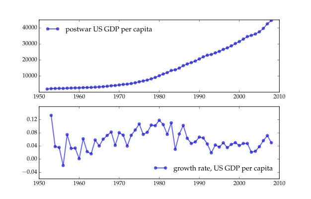
Figure 7.1 shows the evolution of US GDP per capita since the early postwar era. The top panel is per capita GDP itself, while the second panel is the growth rate. How could we go about modeling such time series in a parsimonious way?
Figure 7.1:Postwar US GDP per capita. Source: Penn World Tables
No reasonable model can be deterministic, since shocks play an important role in year-on-year change in GDP, and an IID process is too simple. We can, however, get close to both of these time series with one of the most common nontrivial stochastic processes: the scalar Gaussian AR(1) model
xt+1=b+axt+cwt+1with {wt}∼IIDN(0,1) and x0 given
Here a,b, and c are parameters, while xt is called the state variable. Equation (7.3) is an example of a stochastic difference equation. The process {xt} it defines is called a stochastic process or stochastic recursive sequence. A realization of the process is called a time series.
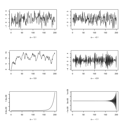
The dynamics of {xt} depends on the parameters. We can get some sense of this from simulation. Six individual time series {xt} are shown in figure 7.2, each generated using a different value of a. The values of b and c are both held fixed at 1, while x0=0. R code for generating the figure is given in listing 3.
As suggested by the figure, the simulated time paths are sensitive to the value of a. If a is outside the interval (−1,1), the series tend to diverge. If ∣a∣<1, then the opposite is true. For example, if you look at the time series for a=0.9 in figure 7.2, you will see that, after an initial burn in period where the series is affected by the initial condition x0, the process settles down to random motion within a band (between about 5 and 15 in this case).
# Generates an AR(1) time series starting from x = init
ar1ts <- function(init, n, b, a) {
x <- numeric(n)
x[1] <- init
w <- rnorm(n-1)
for (t in 1:(n-1)) {
x[t+1] <- b + a * x[t] + w[t]
}
return(x)
}
avec <- c(0.1, -0.1, 0.9, -0.9, 1.1, -1.1)
N <- 200
par(mfrow=c(3,2)) # Arrangement of figures
for (a in avec) {
plot(ar1ts(0, N, 1, a), type="l", xlab=paste("a = ", a), ylab="")
}
If the scalar Gaussian AR(1) model in (7.3) is unable to capture important aspects of a time series that we wish to model, we can generalize it in several different directions. For example, we can remove the assumption that the shocks are normally distributed, in which case it is simply called the scalar AR(1) model. This might be desirable, if, say, the state process has heavy tails.
We can also generalize the scalar AR(1) model to RK, yielding the vector AR(1) model, or VAR(1) model
Here {wt} is assumed to be IID and to satisfy Ewt=0 and E[wtwt′]=I. If wt is multivariate normal, then (7.4) is called the Gaussian VAR(1). The vector xt is called the state vector. A huge variety of models can be represented as a VAR(1) process or contain VAR processes as subcomponents (e.g., linear state space models).
An alternative generalization of the scalar AR(1) model is the scalar AR(p) model, where the next state xt+1 is a linear function not just of the current state xt, but of the last p previous states. For example, the AR(2) process has dynamics
xt+1=b+axt+γxt−1+wt+1
Although xt+1 is a function of two lagged states, xt and xt−1, we can reformulate it as a first-order model. To begin, we define an additional state variable yt via yt=xt−1. The dynamics can then be expressed as
xt+1yt+1=b+axt+γyt+wt+1=xt
We can write this in matrix form as
(xt+1yt+1)=b(10)+(a1γ0)(xtyt)+(10)wt+1
This is a special case of the VAR(1) model in (7.4). This example shows how higher order processes can be reduced to first-order processes by increasing the number of state variables. For this reason most theoretical discussion below takes place in the context of first-order models.
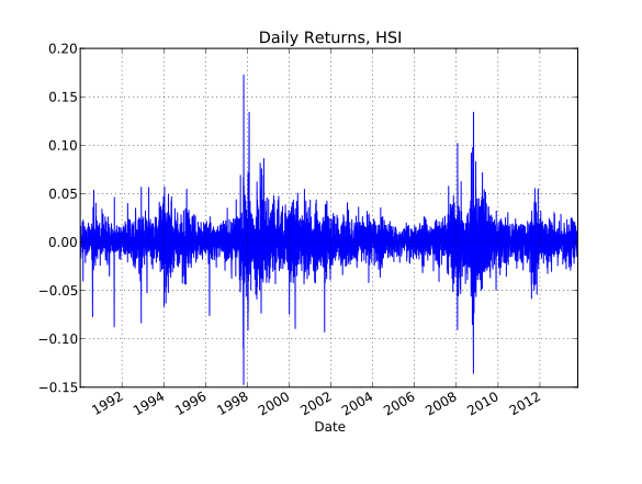
Linear models are simple but that isn’t always an advantage. Sometimes they are unable to capture the kinds of dynamics we observe in data. For example, the bursts of volatility in the graph of daily returns on the Hang Seng Index from 1990 to 2014 shown in figure 7.3 are difficult to replicate without introducing nonlinearities into our model. It’s also true that many theoretical modeling exercises produce models that are nonlinear.
Figure 7.3:Daily returns on the Hang Seng Index. Source: Yahoo! Finance
One well-known nonlinear model is the pth order autoregressive conditional heteroskedasticity model (ARCH(p) model). The model arose from the need to attach a time varying volatility component σt to asset return models. Suppose, for example, that xt=σtwt where σt+12=α0+α1xt2. Combining these equations gives the ARCH(1) model
Here τ:R→[0,1] is increasing and satisfies lims→−∞τ(s)=0 and lims→∞τ(s)=1. For s near −∞, g(s) is similar to b0+a0s. For s near +∞, g(s) is close to b1+a1s. Thus the dynamics transition between two different linear models, with the smoothness of the transition depending on the shape of τ.
All of the examples in Section 7.1.2 are special cases of a general class of process called Markov processes. Markov processes are very rewarding to study because the concepts are broad enough to include a vast array of different stochastic processes, while at the same time having enough structure to support elegant and powerful theory. Here we cover the foundations, from definitions and basic properties to stability and asymptotics.
Let S be a subset of RK and let B(S) be the Borel subsets of S. The fundamental primitive of a discrete time Markov process on S is a stochastic kernel or transition probability function, which is a function Q:S×B(S)→[0,1] such that
Q(s,⋅) is a probability measure over B(S) for all s∈S and
g(s):=Q(s,B) is B-measurable for each B∈B(S).
S is called the state space of the model. Part (ii) is a mild regularity condition that ensures certain integrals are well defined. Part (i) is the major defining characteristic, yielding a distribution supported on S for every point s in S. We think of Q and some initial distribution P0 as generating a corresponding Markov process {xt} taking values in S via
draw x0 from P0
fort in 0,1,2,…do
draw xt+1 from the distribution Q(xt,⋅)
end
The value Q(s,B) is then the probability that xt+1 lands in B given xt=s. The sequence {xt} so generated is also called a sample path for Q.
There is a measure-theoretic procedure for building this process {xt} more formally but the construction is usually unnecessary because most Markov processes are introduced via a stochastic difference equation, which specifies both the process {xt} and, implicitly, the associated stochastic kernel Q. The canonical stochastic difference equation for a first-order Markov process takes the form
Here {wt}t⩾1 is an IID sequence of RM-valued shocks with common distribution Ψ and G is a given B-measurable function mapping the current state xt∈S and shock wt+1∈RM into the new state xt+1∈S. The initial condition x0 and the shocks {wt}t⩾1 are also assumed to be independent of each other. The corresponding stochastic kernel is
Q(s,B)=P{G(s,wt+1)∈B}(s∈S,B∈B(S))
The choice of date t+1 is irrelevant here because of the IID assumption, and is used only to tie in with (7.7). Recalling that Ψ is the distribution of wt+1, the stochastic kernel can also be written as
Q(s,B)=Ψ{w∈RM:G(s,w)∈B}
This expression makes it clear that Q is defined by the two primitives G and Ψ.
Returning to the general process (7.7), repeated substitution gives
and so on. Continuing in this fashion, we see that the state vector xt can be written as a function of x0 and the shocks w1,…,wt for any t. In other words, for each t, there exists a function Ht such that
Often there is no neat expression for the function Ht. Nonetheless, (7.8) clarifies the fact that (7.7) pins down each xt as a well-defined random vector, depending on the initial condition and the shocks up until date t. Since xt is a function of x0,w1,w2,…,wt, and these random vectors are all, by the IID assumption, independent of wt+k for any k⩾1, fact 5.1.10 tells us that the current state xt and future shocks are independent. Let’s record this:
Although it’s rarely made explicit, behind all the random vectors {xt} lies a single probability space (Ω,F,P). The idea is that an element ω of Ω is selected by “nature” at the start of time. This determines the initial condition x0 and the shocks wt as
x0(ω),w1(ω),w2(ω),w3(ω),…
From these, each state vector xt is determined via
In other words, q(s,⋅) is the conditional density of xt+1 given xt=s. Heuristically, q(s,s′)ds′ is the probability of transitioning from s to s′ in one step.
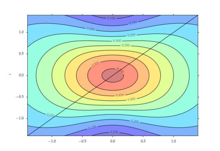
A visualization of the ARCH kernel (7.11) is given in figure 7.4 when α0=0.5 and α1=0.8. The diagonal line is the 45 degree line. Each vertical fiber of the graph corresponds to one density s′↦q(s,s′). For large s (to the right on the horizontal axis), the corresponding density puts most mass below the 45 degree line, indicating a tendency to decrease. Conversely, when −s is large, the process tends to increase.
Let’s note some features of the marginal and joint distributions of a Markov process. Consider our generic process xt+1=G(xt,wt+1) from (7.7), where L(x0)=P0 and {wt} is IID on RM with common distribution Ψ. The marginal distribution of the state vector is just L(xt). Since xt is a well-defined random vector (see in particular (7.8)), L(xt) is also well-defined, and we denote it in what follows by Pt. That is,
Pt(B)=P{xt∈B}(B∈B(S))
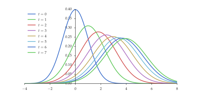
Figure 7.5 shows a visualization of this sequence when μ0=0, σ0=b=c=1 and a=0.8. In fact we don’t actually need to recompute the sums in the definition of μt and σt2 at each step because these sequences satisfy the recursions
You can verify this by taking expectations and variances on both side of (7.3).
Figure 7.5:Sequence of marginal densities for the Gaussian AR(1) process
For a general Markov process, tracking evolution of the first two moments is usually more complicated, and even then fails to provide full information on the distributions. We do, however, have the following general result:
Exercise 7.6.4 asks you to prove this. Fact 7.2.2 is a version of the law of total probability . To calculate the probability of reaching B next period, we sum the probability of that event given outcome s today, weighted by the probability that s occurs today. Here’s a parallel result for the density case.
Let’s now look at joint distributions. We’ll cover these only in the density case, which is the most important case in econometrics.
This result can be obtained in a few different ways. One is to repeatedly apply (5.27) to factor the joint density into
pT(s0,…,sT)=p0(s0)t=0∏T−1p(st+1∣st,…,s0)
This is the expression for the joint density of a general stochastic process, where the current state depends on lagged states of all orders. With the first-order Markov property, an expression like p(st+1∣st,…,s0) reduces to p(st+1∣st), which is just q(st,st+1).
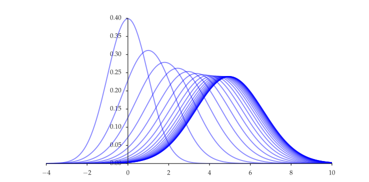
Consider the notion of stationarity introduced in Section 7.1.1. Not every Markov process is stationary. As stated above, a necessary condition is that the marginals are constant, and in figure 7.5 we saw an example of how the marginals {Pt} can change over time. Figure 7.6 shows the same sequence but now longer, with identical parameters. Probability mass moves from left to right.
Figure 7.6:Convergence of marginal densities, Gaussian AR(1) case
While {Pt} is not typically constant, for the particular sequence shown in figure 7.6, the difference between successive distributions is diminishing over time. We can see this analytically as well by recalling that Pt=N(μt,σt2), where μt and σt2 are as given in (7.14). Provided that ∣a∣<1, these sequences converge, with
μt→μ∞:=1−abandσt2→σ∞2:=1−a2c2
Let P∞ denote the distribution associated with these limits. That is,
What happens if we actually attain this limiting distribution, or if we take our initial draw x0 from this distribution? On an intuitive level, it seems that the distribution sequence will be constant, remaining at P∞ over time. Indeed this is the case, as exercise 7.6.1 asks you to confirm.
The limiting distribution is an example of what is called a stationary distribution. More generally, a stationary distribution for a Markov process on S with stochastic kernel Q is any distribution P∞ on S satisfying
P∞(B)=∫Q(s,B)P∞(ds)for all B∈B(S)
Comparing with the recursion Pt+1(B)=∫Q(s,B)Pt(ds) from fact 7.2.2, we see that the definition of stationarity of P∞ means precisely that
L(xt)=P∞⟹L(xt+1)=P∞
From this we see that any process starting at P∞ will be identically distributed. In fact it is stationary, in the sense that (7.1) holds. Let’s record this:
Moments of the stationary distribution are called the stationary moments of the Markov process. Other names for the stationary distribution include the "invariant" or "unconditional" distribution, and the moments are then called the invariant or unconditional moments.
Not every Markov process has a stationary distribution. For example, in the linear scalar AR(1) model xt+1=b+axt+cwt+1, we know that the marginal variance evolves according to σt+12=a2σt2+c2. If ∣a∣⩾1, then this sequence diverges. Because the variance is not constant, the distribution sequence cannot be constant either.
Let’s state one sufficient condition for existence. The condition we give slightly specializes a famous result known as the Krylov–Bogolyubov theorem. It uses the notion of a coercive function, which is any nonnegative function V on the state space S such that
Cγ:={s∈S:V(s)⩽γ}
is a compact subset of S for all γ∈R. Intuitively, coercive functions are functions that go to +∞ as we move "away from the center" of the state space.
Now we can state the following:
See §11.2 of Stachurski (2009) for proofs and references. Condition (7.20) is an example of a drift condition. One way to understand it is to write it as
V(s)EV[G(s,wt+1)]⩽λ+V(s)L
As we move "away from the center" of the state space, V(s) becomes large, and the term on the right is eventually <1. Looking at the left hand side, this tells us that the value attached to the state by V is expected to decrease, which in turn suggests movement away from the "edges" of the state space and back towards the center.
When do Markov processes exhibit nice properties such as ergodicity? To gain some intuition, let’s first consider the process xt+1=axt+wt+1, where {wt} is IID N(0,1) and ∣a∣<1. We consider a stationary process, where each xt has marginal
Thus, to obtain varxˉT→0 as T→∞, we require the covariance terms E[xt+jxt] to converge to zero in j sufficiently quickly. That they do in this particular instance is the subject of exercise 7.6.3.
To summarize, if correlations die out sufficiently quickly, then we can regain the LLN. The same is true for the CLT when second moment conditions hold. We now state a much more general result for sample paths of Markov processes. The proofs are omitted but the essential ideas are the same.
Conditions (a) and (b) are not dissimilar to the conditions for existence in theorem 7.2.1. Condition (b) is the drift condition in (7.20) specialized to the density setting. The major difference is that q is required to be strictly positive. This gives enough mixing to generate uniqueness and the sample path properties. Theorem 7.2.2 can be proved from results in Meyn & Tweedie (2009).[1]
Theorem 7.2.2 is but one of a vast range of results on asymptotic properties of Markov processes. Discussion of alternatives is given in Section 7.5. In fact the conditions are rather strict and can certainly be weakened at the expense of a more complex theorem statement. Nonetheless, they suffice for many applications of interest.
The constant σh2 in (7.27) is given by the expression
with the understanding that {xt} is a stationary process. If σh2=0, then the limiting distribution is degenerate.
To see why, recall from (7.13) that the transition density satisfies q(s,s′)=ψ(s′−g(s)). Since ψ is assumed continuous and positive on RK, the transition density has these properties on RK×RK. Hence condition (a) in theorem 7.2.2 is satisfied. Condition (b) is also satisfied because, taking λ and L as in (7.29), we have
∫∥s′∥q(s,s′)ds′=E∥g(s)+wt+1∥⩽λ∥s∥+L+∫∥w∥ψ(w)dw
For most Markov processes the stationary density has no known closed-form. However, in the case of example 7.2.11, the stationary density is known to have the form p∞(s)=2ϕ(s)Φ(qs), where q:=a(1−a2)−1/2, ϕ is the standard normal density and Φ is the standard normal CDF.
where {wt} is assumed to be IID and to satisfy Ewt=0 and E[wtwt′]=I. Regarding the asymptotics of this process, if the shock vector has a continuous and positive density, then we can apply fact 7.2.7 to obtain asymptotic stability and LLN and CLT results whenever the matrix norm of A satisfies ∥A∥<1. To see this, let g(s)=b+As. By the norm triangle inequality and the definition of the matrix norm, we have
As mentioned above, the stability and sample path conditions considered above are relatively strict. In the linear case, we can certainly do better. Here’s one such result:
Here ϱ(A) is the spectral radius of A, as defined. Under this condition, a unique stationary distribution exists. Taking expectations across (7.30), we see that its mean μ∞ must satisfy μ∞=b+Aμ∞. Applying the Neumann series lemma, this equation has the unique solution
μ∞=(I−A)−1b=i=0∑∞Aib
Let Σ∞ be the asymptotic variance (i.e., the variance–covariance matrix of the stationary distribution). From (7.30) it must satisfy
Σ∞=AΣ∞A⊺+CC⊺
This is an example of a discrete time Lyapunov equation. Under the condition ϱ(A)<1 it can be solved by iteration or by using existing numerical solvers. Here’s an example in Julia that uses a solver from the QuantEcon package:
using QuantEcon
A = [0.8 -0.2;
-0.1 0.7]
C = [0.5 0.4;
0.4 0.6]
solve_discrete_lyapunov(A, C * C')
Martingales generalize the notion of a random walk, where increments to the current state are draws from a white noise process. The concept of martingales has been central to many advances in probability since the mid twentieth century. Econometricians also like martingales because they neatly capture the idea of "unpredictable" change.
To define martingales, we need the notion of a filtration, which is an increasing sequence of information sets. Recall from Section 5.2.4 that an information set is just a set of random variables. Let {Ft} be a sequence of information sets. That is, Ft is an information set for each t. The sequence {Ft} is called a filtration if, in addition, Ft⊂Ft+1 for all t. Intuitively, expanding information sets reflect the idea that more information is revealed over time.
Now let {mt} be a scalar stochastic process and let {Ft} be a filtration. We say that {mt} is adapted to {Ft} if mt is Ft-measurable for every t. (For the definition of measurability, see Section 5.2.4.)
The intuitive meaning is this: Ft represents the variables we know as of time t. If {mt} is adapted to Ft, then we can compute mt at time t as well.
The proof goes like this: By adaptedness, mt is Ft-measurable. From the definition of a filtration we have Ft⊂Ft+j. Applying fact 5.2.10, it follows that mt is Ft+j-measurable. Fact 7.3.1 now follows from fact 5.2.13.
A sequence of integrable random variables {mt} adapted to a filtration {Ft} is called a martingale with respect to {Ft} if
E[mt+1∣Ft]=mtfor allt
The expression E[mt+1∣Ft] is sometimes simplified to Et[mt+1] when the filtration is understood.
Next we consider asymptotics for martingale difference sequences. Such sequences are good candidates for the LLN and CLT. To see this, recall that integrable IID sequences always satisfy the LLN. With finite second moment they also satisfy the CLT. Suppose now that {mt} is a stationary MDS with respect to some filtration {Ft}. We don’t have independence in this case but we do have the following:
To see this, fix t⩾0 and j⩾1. We have
cov[mt+j,mt]=E[mt+jmt]=E[E[mt+jmt∣Ft+j−1]]
Since t+j−1⩾t and {Ft} is a filtration, we know that mt is Ft+j−1-measurable. Hence
The lack of correlation in fact 7.3.3 is a key part of the next result.
The proof of (7.32) is identical to that of the classical LLN in theorem 6.1.1. Theorem 7.3.1 can be established from a martingale CLT proved in Durrett (2010).
Simulation is invaluable as a tool for exploring statistical concepts and solving applied problems. For example, the current popularity of Bayesian methods for econometrics and machine learning has been driven to a large extent by clever simulation algorithms that have proved successful at solving hard estimation problems.
Modern scientific programming environments all have good routines for simulating independent observations from a range of common named distributions. We’ve seen examples of this in the displayed computer code. But it’s easy to run into situations where the distribution we are working with is nonstandard, or has no closed-form solution. We then need to roll our own routines for producing random variates. Let’s review two of the most important algorithms.
Suppose that we wish to draw from a distribution on R with CDF F. Assuming that we can generate uniform random variables, we can do so via the inverse transform method:
draw u from the uniform distribution on [0,1]
return F−1(u), where F−1 is the quantile function of F (see (4.35))
We wish to show that this technique is valid, or, equivalently, that
In the proof we’ll assume that F is strictly increasing. (This isn’t necessary, but the proof of the general case provides no additional intuition.) Let L(u)=U[0,1] and let z:=F−1(u). To see that L(z)=F, observe that, by strict monotonicity, F(a)⩽F(b) if and only if a⩽b. As a result, for any s∈R,
P{z⩽s}=P{F−1(u)⩽s}=P{u⩽F(s)}
The defining property of a U[0,1] random variable u is that P{u⩽t}=t whenever 0⩽t⩽1. Using this fact in the preceding calculation gives P{z⩽s}=F(s), proving (7.34).
Here’s one extension for the basic inverse transform method. Suppose that we want to simulate from a joint distribution on RN that is defined in terms of a copula (see Section 5.1.5). In particular, suppose that Fn is a continuous CDF on R for n=1,…,N, that C is a copula on RN and that the joint distribution of interest is
F(s1,…,sN)=C(F1(s1),…,FN(sN))
(This is just (5.22).) If we can simulate from C, then we can simulate from F. The method is
draw u1,…,uN from C
return (x1,…,xN):=(F1−1(u1),…,FN−1(uN))
Exercise 7.6.13 asks you to prove that (x1,…,xN) is a draw from F.
Markov chain Monte Carlo (MCMC) is a way of simulating from a given density π on S⊂RK. The idea is to construct a stochastic kernel P on S such that
π is a stationary distribution for P, and
P is sufficiently ergodic that its sample path averages converge to expectations under π
See (7.26) for a clearer statement of (ii). If we specialize to indicator functions we can approximate probabilities under π too.
There are two major strands of MCMC algorithms: Metropolis–Hastings and the Gibbs sampler. Here we’ll cover the former. While boldface symbols are omitted in what follows, the ideas are valid in any dimension. In the section on Bayesian estimation in Section 8.3.4, I will explain why Metropolis–Hastings fits so beautifully with Bayesian updating.
The Metropolis–Hastings algorithm starts with a Markov process in the form of a stochastic density kernel q=q(s,s′) called the proposal density. Draws from the proposal density are called proposals. Each time we draw a proposal, we either (i) accept it and move to that new state, or (ii) reject it and stay put. The probability of accepting is structured so that the chain tends to stay in regions where π puts most probability mass. As a consequence, for a sequence {xt} generated by this process, we get
fraction of time spent in B=T1t=1∑T11{xt∈B}≈π(B)for large T
The ideas are subtle, so let’s build up in steps. Consider first a general accept-reject style process of the kind discussed above, where the probability of acceptance is determined by an arbitrary function α=α(xt,y) of the current state xt and proposal y. The function takes values in [0,1]. The algorithm for generating xt+1 from xt given α and proposal density q is given in algorithm 1.
The stochastic kernel P associated with {xt} in algorithm 1 has the form
To show this, we can break the probabilities up as follows. Fix any Borel set B and let xt be given at s. Let xt+1 be drawn according to algorithm 1 when xt=s. By additivity of P we can write P{xt+1∈B} as
Our aim is to show that the two terms in (7.36) match the two terms on the right-hand side of (7.35).
Using the fact that intersections become products when we switch to indicators (fact 4.1.4, page ), we can applying the law of iterated expectations to obtain
The term E[11{u⩽α(s,y)}∣y] is just P{u⩽α(s,y)} with y given, which, since u is uniform, evaluates to α(s,y). Hence the final expression in the last display evaluates to
Equation (7.37) says that the first term in (7.36) is equal to the first term on the right-hand side of (7.35). For the second terms, note that xt+1=xt=s when u>α(s,y), so
To match this expression with the second term in (7.35), we just need to show that P{u⩽α(s,y)}=∫p(s,s′)ds′. But this is immediate from (7.37) if we take B=S.
So far we have verified that the kernel P in (7.35) is the stochastic kernel corresponding to algorithm 1. Now let’s double back and design the selection function α so that the stationary distribution of P is the target density π. In the Metropolis–Hastings algorithm, this is done by setting
If π(s)q(s,s′)=0, then α(s,s′):=1. The min is in place so α(s,s′) can be interpreted as a probability. We don’t actually need to impose it in algorithm 1, since for u∈[0,1] we have u⩽min{a,1} iff u⩽a. The important element is the ratio inside the min, which is large when the new proposal s′ has high probability under π relative to the current location s and small when the reverse is true. This keeps the chain in regions where π has high mass, and leads to our next result.
It remains to establish that P has the kind of stability properties discussed in theorem 7.2.2 (and in particular the LLN result in (7.26) of that theorem). This isn’t universally true, and requires at least some conditions on the primitives q and π. One well-known result is given in corollary 3 of Tierney (1994) for the case where q and π are continuous and strictly positive on S and S itself is compact. In essence, the continuity and positivity corresponds to condition (a) of theorem 7.2.2, while the compactness of S is a strict version of the drift condition in (b) of the same theorem.[3] For further results and references, see Roberts et al. (2004).
One disadvantage of MCMC methods is that the variates they generate are not in general independent. Sample averages from dependent samples are typically less informative than IID samples. (See example 7.1.4 for the extreme case.) It is desirable, then, that dependence between xt and xt+k dies out quickly as k increases. Whether it does or not is determined by the choice of q. Extensive discussion of such issues can be found in Brooks et al. (2011).
A function implementing the Metropolis–Hastings algorithm in Julia with a random walk proposal density is given in listing 4. The proposal density takes the form q(s,s′)=ψ(s′−s), where ψ is a given density. This is the system (7.12)–(7.13) with g set to the identity. If ψ is symmetric, then q(s,s′)=q(s′,s), and α(s,s′) simplifies to min{π(s′)/π(s),1} if π(s)>0 and 1 otherwise. This is the case shown in listing 4, with ψ set to the N(0,σ2) distribution. Look up Julia’s ternary operator if you find it hard to follow the code.
function rw_metropolis(pi_density, T, init=0, sigma=1)
xvec = Vector{Float64}(undef, T)
xvec[1] = init
for t in 1:(T - 1)
x = xvec[t]
y = x + sigma * randn()
alpha = pi_density(x) > 0 ? pi_density(y) / pi_density(x) : 1
xvec[t+1] = rand() < alpha ? y : x
end
return xvec
end
Listing 4:The random walk Metropolis–Hastings algorithm (Julia)
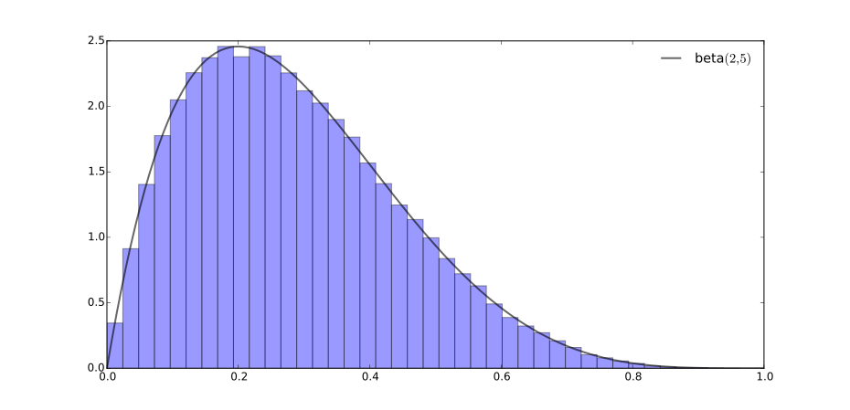
Figure 7.7 shows a histogram of 106 draws generated from this algorithm when π is the beta distribution with parameters (2,5). The black line is the target density. This is just a toy example, since routines for sampling from beta distributions are readily available.
Figure 7.7:Observations from the random walk Metropolis–Hastings algorithm
The modern theory of Markov processes owes much to a brilliant mathematician called Wolfgang Doeblin. His short life and shining contributions to probability theory are discussed in Bru & Yor (2002).
An excellent overview of Markov processes and their stability can be found in Meyn & Tweedie (2009). For more on Markov processes from a density perspective see Lasota & Mackey (1994) or chapter 8 of Stachurski (2009). For a nice survey of sample path properties with a focus on the central limit theorem, see Jones (2004).
Diaconis (2009) provides a fascinating overview of MCMC and its impact on different fields. Richey (2010) is a more general survey. Good references on the theoretical side include Roberts et al. (2004), Tierney (1994), and Geweke (1996). See Kroese & Chan (2014) for a more practical discussion with a focus on applications.
The stated results are a consequence of theorem 17.0.1 in Meyn & Tweedie (2009), which in turn requires that the process is V-uniformly ergodic. In our case, the latter property follows from aperiodicity and irreducibility, which are immediate consequences of strict positivity of q on S×S, and from the drift condition (b). In the language of Meyn & Tweedie (2009), the function V is "unbounded off petite sets." This holds for any coercive function V when q is positive and continuous, since compact sets are then petite.
Stachurski, J. (2009). Economic Dynamics: Theory and Computation. Cambridge: MIT Press.
Meyn, S. P., & Tweedie, R. L. (2009). Markov Chains and Stochastic Stability (2nd ed.). Cambridge, UK: Cambridge University Press.
Hall, R. E. (1978). Stochastic implications of the life cycle-permanent income hypothesis: theory and evidence. Journal of Political Economy, 86(6), 971–987.
Durrett, R. (2010). Probability: Theory and Examples (4th ed.). Cambridge, UK: Cambridge University Press.
Tierney, L. (1994). Markov chains for exploring posterior distributions. The Annals of Statistics, 22(4), 1701–1728.
Roberts, G. O., Rosenthal, J. S., & others. (2004). General state space Markov chains and MCMC algorithms. Probability Surveys, 1, 20–71.
Brooks, S., Gelman, A., Jones, G., & Meng, X.-L. (2011). Handbook of Markov Chain Monte Carlo. Boca Raton: CRC Press.
Bru, B., & Yor, M. (2002). Comments on the life and mathematical legacy of Wolfgang Doeblin. Finance and Stochastics, 6(1), 3–47.
Lasota, A., & Mackey, M. C. (1994). Chaos, Fractals, and Noise: Stochastic Aspects of Dynamics (Vol. 97). New York: Springer.
Jones, G. L. (2004). On the Markov chain central limit theorem. Probability Surveys, 1, 299–320.
Diaconis, P. (2009). The Markov chain Monte Carlo revolution. Bulletin of the American Mathematical Society, 46(2), 179–205.
Richey, M. (2010). The evolution of Markov chain Monte Carlo methods. American Mathematical Monthly, 117(5), 383–413.
Geweke, J. (1996). Monte Carlo simulation and numerical integration. In Z. Griliches, R. F. Engle, & M. D. Intriligator (Eds.), Handbook of Computational Economics (Vol. 1, pp. 731–800). Elsevier.
Kroese, D. P., & Chan, J. C. (2014). Statistical Modeling and Computation. New York: Springer.