In probability theory we aim to deduce the likelihood of different outcomes based on known probability distributions. Statistics is the inverse problem. We want to infer unknown probability distributions from outcomes we observe. In this chapter we begin to explore these ideas.
8.1The Estimation Problem¶
Let’s start off by clarifying the nature of the problem we want to study.
8.1.1Definitions¶
From a pedagogical point of view, it’s best to start our study of statistics in a setting where successive observations are both independent and identically distributed. Later we’ll extend to dependent data. In an IID setting, the fundamental problem of econometrics and statistics is this:
The set is the universe of distributions we are willing to consider. It can be anything, including the set of all distributions on the outcome space. One of the main tasks of economic theory is to restrict and thereby narrow down the set of distributions we have to search over.
Let’s set out some notation:
is the outcome space where each observation takes values.
denotes the sample or data set .
is the sample space in which takes values.
is the joint distribution of the sample.
Although calling the sample space follows standard nomenclature, we are overloading the terminology first used. (Unfortunately, statisticians and probabilists don’t always coordinate on terminology.)
As above, is the common distribution of the observations. For as long as we continue to focus on IID data, the joint distribution will be the th product of , as defined.
the mean and higher moments of ,
measures of dispersion, such as the variance, or properties of tails,
the median and other quantiles, and
itself, or the density of if it exists.
In example 8.1.2, the individual observations are scalar. In other scenarios, observations are vector-valued:
Because the marginal distribution of the observations is now multivariate, new features of the distribution come in to play, such as
correlations across coordinates of ,
the variance–covariance matrix associated with , and
parameters controlling dependence when, say, is modeled via a copula over certain marginals.
8.1.1.1Features¶
We referred above to "features" of that we might be interested in estimating. Let’s define a feature of to be an object of the form
The set is left arbitrary to accommodate all possible features. When is understood, we’ll write as . Here are some examples for univariate routinely estimated in econometric studies:
, the th moment of .
, the median of .
, when we want to estimate itself.
the density of when is absolutely continuous.
If is multivariate over , then one feature of interest is the regression function . This function is uniquely determined by (see Section 5.2.5).
8.1.1.2Parametric versus Nonparametric Classes¶
In the statistical problems listed above, it is assumed that the unknown distribution belongs to some class . We call a parametric class if it can be expressed as
In other words, a class of distributions is parametric if it can be indexed by finitely many parameters. A class of distributions is called nonparametric if it is not parametric.
Many traditional methods of inference are parametric in nature: The data are assumed to be generated by an unknown element of a parametric class . The aim is to estimate using the data. Once we have an estimate of , we can plug this estimate back into the parametric class to obtain an estimate of .
The concept of a feature defined in (8.1) is a generalization of the notion of a parameter or vector of parameters. In parametric settings, the feature that we are most interested in estimating is the parameter vector . If we have a good estimate of , we can estimate any feature via .
Following common usage, we will sometimes refer to the associated with the that generates the data as the true value of the parameter vector. However, it’s important to remember that this is an assumption, not a "truth." We assume that the data are generated by some member of a parametric class. This assumption can be completely false.
In our initial formulation of the estimation problem we considered estimation of features rather than just parameters because it is suboptimal to always restrict ourselves to parametric assumptions on . We’ll discuss the relative merits of parametric and nonparametric estimation more in chapter 14.
8.1.2Statistics and Estimators¶
A statistic is any observable function of the data. More precisely, a statistic is any -measurable function
that can be evaluated once the data are observed. As in (8.1), the set is left arbitrary to accommodate all the possible features that we might wish to estimate. Sometimes we write as to emphasize dependence on the sample size. The assumption that a statistic is -measurable is just a basic regularity condition.
An estimator is a statistic used to infer some feature of an unknown distribution . Thus a statistic becomes an estimator when paired with and compared to a feature of the distribution. Note that there is nothing in the definition of an estimator that implies it will be a sensible estimator of the target feature, let alone a good one.
julia> using Statistics; median([1, 3, 5])
3.0
julia> median([2, 4, 6, 8])
5.0In some texts the sample variance is defined as rather than (8.2) in order to produce an unbiased estimator. However, (8.2) fits better with the theory in this text and is perhaps the more common definition.
8.1.3Empirical Distributions¶
The empirical distribution of a given -valued sample is the discrete distribution on that puts equal probability on each sample point . Another way to state this is that assigns to each Borel set the number
This is just the fraction of the sample that falls in . (Refer back to figure 4.2 if you wish to see a visual representation.) The expectation of a function with respect to is
as follows from (5.14).
The empirical distribution is a statistic, mapping observations into , a random element of the set of all distributions on . If we think of as independent draws from common but unknown distribution , then becomes an estimator of . In particular, if the feature of we want to infer is itself, the simplest natural estimator is the empirical distribution.[1]
With scalar data we can visualize the empirical distribution by plotting its CDF. The CDF of will be denoted in what follows by . Specializing in (8.7) to , we get
The CDF is called the empirical cumulative distribution function, or ECDF, corresponding to the sample. Graphically, is a step function, with an upward jump of at each data point. Figure 8.1 shows an example where draws are from the CDF of the Beta distribution. Each panel shows an observation of the ECDF, which is in turn constructed from observations from .
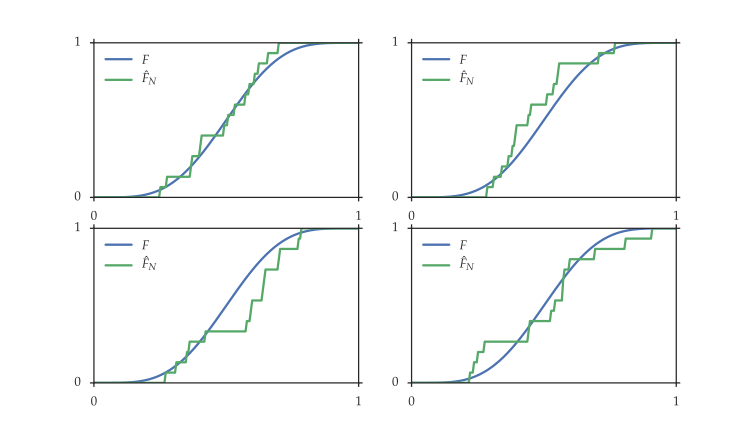
Figure 8.1: and four observations of when
8.1.3.1Convergence¶
The empirical distribution is asymptotically an excellent estimator of . If are IID with common distribution and is the empirical distribution, then, by the law of large numbers,
for any Borel set . See, in particular, (6.8).
Specializing to the scalar case with , we have for any , where is the CDF of . In fact a much stronger statement is also true. It is sometimes called the fundamental theorem of statistics, or the Glivenko–Cantelli theorem:
The norm here is the supremum norm, meaning that
Roughly speaking, this is the maximal deviation over the domain. (For a definition of the supremum, see Section 15.4.1.) In fact the convergence occurs “almost surely,” which is a stronger notion than in probability. See theorem 11.4.2 of Dudley (2002).
Figure 8.2 illustrates the convergence in (8.11). Each ECDF is based on a single sample of independent draws from , where is Beta. Each subplot shows 8 realizations of the ECDF at a different value of . Across the subplots, the sample size is stepped up from 10 to 500.
Theorem 8.1.1 tells us that, at least in the IID setting, if we have an infinite amount of data, then in the limit we can learn the underlying distribution without having to impose any assumptions at all. Moreover, once we know the distribution , we know any feature .
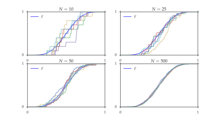
Figure 8.2:Realizations of with four different sample sizes
Does this offer a solution to the basic problem of estimation stated? The answer is no. In practice, we only ever have a finite amount of data. Inference is about generalization, as discussed in the introduction. There’s no need to generalize if we know the full population.
Moreover, when we still have only finitely many observations, the empirical distribution puts all of its mass on these points. In other words, it treats the sample like the unknown distribution, without acknowledging the fact that we have limited information. This can be viewed as an extreme form of overfitting. We’ll discuss related ideas in a number of contexts throughout the book.
8.1.3.2Identification¶
A class of distributions indexed by is called identifiable if the map is one-to-one (see Section 15.2) on .
Identifiability means that the parameter vector associated with the unknown distribution can eventually be distinguished from the data. To see this, suppose that is identified on and nature generates an infinite sequence of observations from . Let be any other vector in and let . By identifiability, there exists at least one Borel set with . Since the empirical distribution converges to , we can in the limit conclude that the data are not generated by .
8.2Estimation Principles¶
We started off with the problem of estimating a feature of the unknown distribution from a sample. We’ve introduced a number of different statistics aimed at estimating various features. Where do these estimators come from and what, if anything, do they have in common?
8.2.1The Sample Analogue Principle¶
Most of the estimators defined above can be derived from a simple principle. In the modern statistical literature this is often called the plug-in method. In econometrics it goes by a variety of names, including "analogue estimation" (see, in particular, Manski (1986)). We’ll call it the sample analogue principle. The principle is:
Here is the empirical distribution constructed from the sample. We replace the unknown distribution with the observable distribution and then evaluate .
The th sample moment applies the same principle to estimate the th moment.
The estimators in these two examples are relatively straightforward, but the set of all applications of the sample analogue principle is very broad. As we’ll see below, estimation methods that can be obtained as special cases include least squares regression, maximum likelihood, the method of moments, and the generalized method of moments.
8.2.1.1Best Linear Prediction¶
Here’s an example that illustrates the generality of the sample analogue principle. Recall the best linear prediction problem from Section 4.1.5.1, where and are chosen to minimize . Letting be the distribution of , we can write the problem as
There is a corresponding statistical problem when the underlying distribution is unknown. The problem is to produce the best linear predictor based only on a sample of observations from . We proceed as follows: Given , we form the empirical distribution
Applying the sample analogue principle, we plug into (8.12), yielding the estimator
(The term has been dropped from the right-hand side of (8.13) because it doesn’t affect the minimizers.) This is the simple linear bivariate least squares problem. The minimizers are
(See ex. 8.5.2.) Comparing with (4.23), we see that these estimators are themselves the sample analogues of the underlying features and .
8.2.1.2Limitations¶
While the sample analogue principle produces sensible estimators in many situations, there are also instances where it fails completely. Let’s look at one example.
Let be the set of absolutely continuous distributions on , so that the distribution generating the data is assumed to have a density. The density of can be regarded as the feature
Here the derivative of the CDF of .
Let be the empirical distribution from any given sample. What happens when we plug this empirical distribution into the right-hand side of (8.15)? In other words, what information do we get when we differentiate the function ? Since is a step function, the derivative is zero everywhere, except at a finite number of jump points where the derivative is undefined. Thus the density estimate produced by the sample analogue principle is useless. This statement remains true even when is enormous.
One way to understand this outcome is that when we wish to estimate complex objects with finite samples, we need to combine the data with some kind of regularization. Loosely speaking, this means that we penalize complexity in our search for a solution, or impose some kind of "smoothing" a priori. This idea has a long history in the field of numerical methods, where certain inverse problems are unstable, or "ill-posed," and their solution requires regularization.
Regularization is an essential element of statistics too. It says that we should not grant the empirical distribution equal status with the unknown true distribution. That is, we should regard the empirical distribution only as partial information, and seek to combine it with some form of prior information or external theory. Regularization is one application of prior information: It applies the idea that probability mass most likely falls in places other than just the sample points observed so far. We pick up the topic of regularization again in chapter 14.
8.2.2Empirical Risk Minimization¶
Let’s now look at another inductive principle that combines the sample analogue principle with additional structure. The principle is called empirical risk minimization, or ERM. The terminology and main concepts come from the machine learning literature. Nonetheless, many standard estimators in econometrics are special cases of ERM, including maximum likelihood and least squares. The ideas discussed here help to frame these tools as part of a broader set of methods.
Consider a setting where we observe an input to a system, followed by a scalar output . Both are random variables and the joint distribution of is . Our aim is to predict new output values from observed input values. We’ll do this by choosing a function such that is our prediction of once is observed. In the machine learning literature, is called a prediction rule. In economics, is called a strategy or policy function.
Incorrect prediction incurs a loss. The size of this loss is written as . The function is called the loss function. Common choices for the loss function include
the quadratic loss function ,
the absolute deviation loss function , and
the discrete loss function .
Given loss function , we consider choosing so as to minimize the prediction risk, which is defined as the expected loss
Sometimes is also called the expected prediction error.[2] The expectation in (8.16) is computed using the joint distribution of . Sometimes we’ll write to emphasize this.
In a statistical setting we are constrained in our ability to minimize risk by the fact that we cannot evaluate , as this requires knowledge of the joint distribution . Suppose, however, that we have access to data , where each pair is an independent draw from . To make use of the sample, we will apply the sample analogue principle, replacing in (8.16) with the empirical distribution . This produces the new objective function
This function is called the empirical risk. The empirical risk is the prediction risk evaluated under the empirical distribution of the sample rather than the true distribution . Minimizing the empirical risk is called empirical risk minimization (ERM).
There is an additional step. When we choose a decision rule the problem that we actually solve is
We have restricted the domain to a class of functions . This set of functions is called the hypothesis space. Choice of is structure we impose on the estimation problem.
It might seem at first pass that we should set to be the set of all functions . After all, if the risk-minimizing function is not in , as visualized in figure 8.3, then the solution to (8.19) is not equal to , and we are making a suboptimal choice.
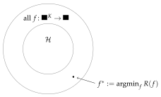
Figure 8.3:Choosing the hypothesis space
Actually this reasoning is false. In fact we usually want to be quite restrictive in our choice of . This is because minimizing the empirical risk is not the same as minimizing the prediction risk. Occam’s razor comes in to play here: we are solving a complex problem on the basis of limited information. It would be a serious mistake to act as if we had unlimited information. These ideas are explored further in Section 8.2.3.
While we ended up with the same minimization problem in two different ways, the reasoning here is more natural. When we first came to this problem in (8.13) it was by applying the sample analogue principle to the problem of finding best linear predictors. Here we are simply trying to find the best predictor. At the same time we have restricted ourselves to linear approximations in recognition of the fact that we are basing our estimate on limited information. Linearity implements Occam’s razor by bounding the complexity of the learning algorithm.
8.2.2.1Quantile Regression¶
Quantile regression is used when we want to estimate a quantile of a given distribution based on a set of predictive variables. For example, quantile regression has been used to estimate quantiles of CEO compensation as a function of the market value of their firms (Koenker & Hallock (2001)). In this section we show how quantile regression can be regarded as a special case of empirical risk minimization.
To describe the idea, let be a strictly increasing CDF on and let be given. Recall from Section 4.2.6 that the th quantile of is the that solves . Although it might not be immediately obvious, the th quantile can also be defined as the solution to the optimization problem
where is a random variable with distribution and
Exercise 8.5.6 asks you to confirm that the solution to (8.23) is precisely the that solves .
Suppose now that we want to estimate the th quantile of using some input variable (e.g., a CEO compensation quantile as a function of firm size). Motivated by (8.23), we can frame the search for a suitable function as a problem of minimizing the prediction risk
where is as defined above. If we employ the principle of empirical risk minimization with data set , we get , where is the hypothesis space. When as defined in (8.21), the ERM problem is
This is the standard expression for the quantile regression problem.
If , then the objective function is proportional to . This case is called median regression or least absolute deviation regression.
8.2.3The Choice of Hypothesis Space¶
Let’s return to the issue of choosing the hypothesis space. We begin with a straightforward result:
In other words, we can always decrease empirical risk by increasing the hypothesis space. The reason that fact 8.2.1 holds is that we are minimizing over a larger set.
At the same time, our actual objective is to minimize the prediction risk. The prediction risk of a given predictor measures the out-of-sample fit of , which is the expected performance of when confronted with new data. A statistical procedure that takes a given data set and produces a predictor with low prediction risk (relative to the benchmark —see (8.17)) means that we have succeeded in meeting the goal we set at the start of the book: we have generalized from data.
Of course, prediction risk is unobservable. Sometimes it is tempting to use empirical risk as an estimator of . However, empirical risk, which measures in-sample fit of , is a downward biased estimator of risk. In particular, as we vary the hypothesis space, prediction risk can rise even when empirical risk is falling.
Let’s illustrate this by way of an example, where empirical risk is minimized over progressively larger hypothesis spaces. The model we will consider is one that generates input-output pairs via
Here is the uniform distribution on the interval . Our hypothesis spaces for predicting from will be sets of polynomial functions. To fix notation, let be the set of all polynomials of degree . That is,
This sequence of hypothesis spaces is increasing, in the sense that
Indeed, if is a polynomial of degree , then can be represented as a polynomial of degree just by setting the last coefficient to zero. The set of linear functions defined in (8.21) is equal to .
If we seek to predict from using quadratic loss and the set as our candidate functions, the risk minimization problem is
while the empirical risk minimization problem is
To illustrate the difference between risk and empirical risk, we first generate data points from the model (8.25). Taking this as our data set, we then solve (8.27) repeatedly, once for each in . The solution to the th minimization problem is denoted , and is, by construction, a polynomial of degree . Finally, we compare the risk and empirical risk .[3] The results are in figure 8.4.
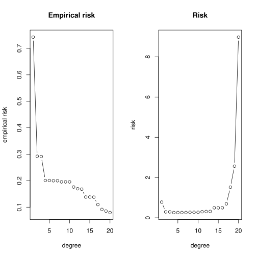
Figure 8.4:Risk and empirical risk as a function of
As expected, empirical risk falls monotonically with . But the risk decreases slightly and then increases rapidly. For large , the minimizer of the empirical risk is associated with very high risk in the sense of large expected loss.
We can get a sense for what is happening by plotting the data and the functions. In figures 8.5–8.8, the data points are plotted alongside the function from the true model (8.25) in black, and fitted polynomial in red. The function is the risk minimizer, and represents the ideal prediction function. In figure 8.5 we have , and the fitted polynomial is the linear regression line. In figures 8.6, 8.7 and 8.8 we have , and respectively. The fitted polynomials are , and .
On the one hand, when , the hypothesis space is small and no function in this class can effectively fit the underlying model. This is called underfitting, and is reflected in the poor fit of the red line to the black line in figure 8.5.
When , the class of functions is considerably larger. Given that the data are relatively noisy, and that we only have 25 observations, the fit of the function is good (figure 8.6). If we look at the risk for on the right-hand side of figure 8.4, we see that it is lower than for .
On the other hand, if we take larger, the fit to the underlying model becomes poor and the risk is high. Examining figures 8.7 and 8.8, which correspond to and , we see that the fitted polynomial has been able to fit the observed data closely, passing near many of the data points. Too much emphasis has been given to this particular realization of the data. When a new input is drawn, the prediction is likely to be a poor predictor of . This situation is called overfitting.
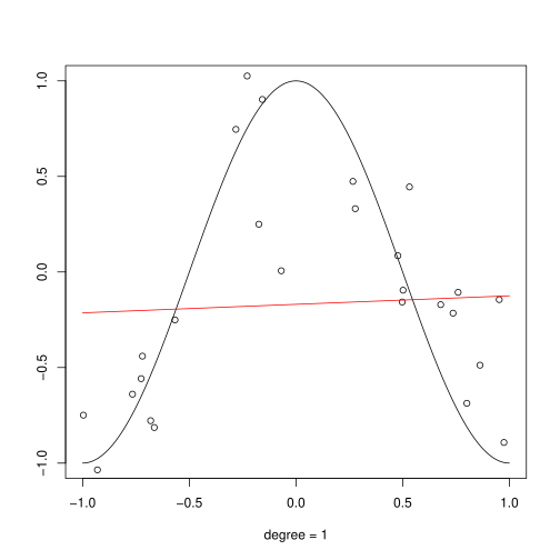
Figure 8.5:Fitted polynomial,
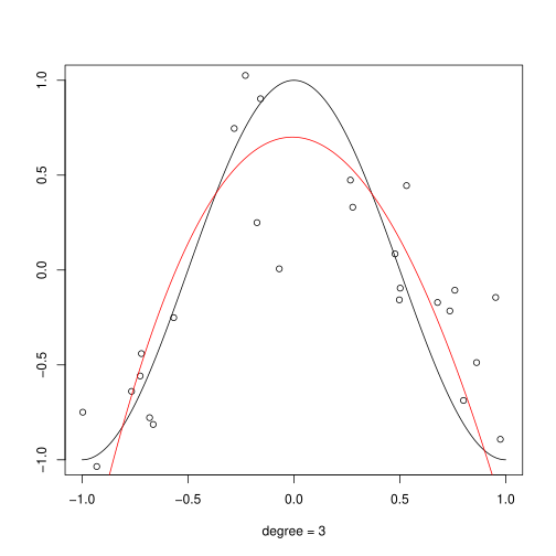
Figure 8.6:Fitted polynomial,
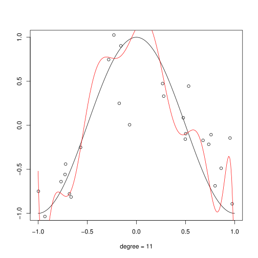
Figure 8.7:Fitted polynomial,
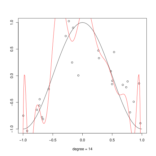
Figure 8.8:Fitted polynomial,
To summarize, the choice of is central to our ability to generalize from the data. When is too small, no function in provides a good fit to the regression function. If this is so, the prediction risk cannot be made small regardless of the data. This can be seen directly from (8.17). Any estimate in must satisfy
Conversely, if is too large, then we can attain low empirical risk but the prediction risk itself is large.
Of course, in statistical applications we do not have the luxury of knowing the true data-generating process when we choose . The best scenario is that we have firm theory that guides us to a suitable hypothesis space. The worst scenario is that we have no idea and choose blindly. Once again, the message is that statistical learning equals prior knowledge plus data.
8.3Some Parametric Methods¶
In this section we review some standard parametric estimation methods, including maximum likelihood, Bayesian estimation, and the generalized method of moments.
8.3.1Maximum Likelihood¶
One standard approach to deriving estimators in a parametric setting is the principle of maximum likelihood. Let’s begin with a simple case and then progress to more complex applications.
Suppose that we observe a single draw from distribution where is unknown. The variance is known and set to for simplicity. Our task is to guess the value of given the observation . A guess of also pins down the distribution , so we could equivalently state that our job is to guess the distribution that generated . In guessing this distribution, if we centered it around some number much larger than , say, then our observed data point would be an “unlikely” outcome for this distribution. See figure 8.9. The same logic would apply if we centered the density at a point much smaller than .[4]
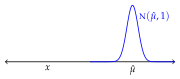
Figure 8.9:Maximizing the likelihood
In fact, in the absence of any additional information, the most obvious guess would be that the normal density is centered on . To center the density on , we just set .
Maximum likelihood formalizes these steps: The density of is the density of the distribution . Plugging the observed value into this density gives
Think of as representing the probability of realizing our sample point . The principle of maximum likelihood suggests that we take as our guess of the value that maximizes this probability. It’s not hard to show that is the maximizer. This coincides with our intuition from figure 8.9.
The same principle applies when the data are independent draws from , where is unknown. The joint density of the sample is the product of the marginals. Plugging the sample values into the joint density, one then maximizes the joint density with respect to :
The maximizer is precisely the sample mean of (see ex. 8.5.4).
We can generalize these ideas in several ways. Let’s suppose now that the data has joint density in the sense of (5.8). We will assume that is a member of a parametric class indexed by parameter vector . Each choice of pins down a particular density , but the value of that generated the data is unknown.
In this setting, the likelihood function is evaluated at the sample , and regarded as a function of :
The principle of maximum likelihood tells us to estimate by maximizing over . A statistic is called a maximum likelihood estimate (MLE) of if
This is equivalent to maximizing the log likelihood function
The set of MLEs can in general be a singleton, contain multiple elements or be empty.
In the preceding discussion, was a density function, but it can be a probability mass function as well. Examples are given below.
To implement maximum likelihood estimation, we need to compute the joint distribution of the data. As we saw in (8.28), when the data points are independent this is easy because the joint density is the product of the marginals. More generally, if each is drawn independently from fixed arbitrary (marginal) density on , then
If each data point is multivariate, just replace with .
Maximum likelihood estimation is a much celebrated theory of estimation. MLE estimators typically have excellent asymptotic properties. But good finite sample properties are not guaranteed (more about this soon) and the attractive asymptotic theory is dependent on correct specification of the underlying parametric class. Indeed we need to bring a lot of knowledge to the table just to form the estimator. (To specify the likelihood function, we must specify the entire joint distribution of the sample.)
8.3.1.1Conditional Maximum Likelihood¶
As in Section 8.2.2, suppose that we observe inputs to some system and corresponding outputs . The pairs are assumed to be IID. Our aim is to estimate in in order to pin down the conditional density of given .
The principle of maximum likelihood tells us to maximize
Letting be the marginal density of , we can use the decomposition (5.27) to write
The density is unknown but we have not parameterized it because we aren’t trying to estimate it. We can now rewrite the log likelihood as
The second term on the right-hand side is independent of and as such it does not affect the maximizer. Hence the MLE is
The objective function here is called the conditional log likelihood. The preceding argument tells us that, when we want to estimate parameters in the conditional density of given , we can maximize the conditional log likelihood directly, which is simpler and more direct than maximizing the full log likelihood.
To find the MLE in this example, we can differentiate to obtain first order conditions, but this does not in general lead to an analytical solution. Instead, numerical optimization of the likelihood is required. Discussion of numerical optimization is given in Section 13.2.2.
8.3.2Maximum Likelihood via ERM¶
Maximum likelihood is a special case of empirical risk minimization. To see this, suppose that we wish to learn unknown density on the basis of observations from . We take our loss function to be
The meaning is this: if our guess of is and the value is realized, then our loss is . Thus we suffer large loss when puts small probabilities near where is realized. The corresponding risk function is
Now suppose that we observe IID draws from . To estimate , the ERM principle indicates we should solve for
where is a hypothesis space of densities. To clarify the connection with maximum likelihood, take to be a parametric class . Choosing our estimate of now reduces to choosing an estimate of . Rewriting our optimization problem for this case, we obtain
Here is the log-likelihood. It follows from this expression that the ERM estimator is precisely the maximum likelihood estimator.
Incidentally, the minimizer of the true risk is the unknown density . To see this, let us first transform our expression for the risk function to
The term on the far right is called the entropy of , and does not involve . Hence minimization of the risk comes down to minimization of
This quantity is called the Kullback–Leibler (KL) deviation between and . The KL deviation is possibly infinite, always nonnegative, and zero if and only if .[5] It follows that the unique minimizer of the risk is the true density .
8.3.3The Method of Moments and GMM¶
Suppose that we wish to estimate a vector that solves an equation of the form
In this expression, and are observable vector-valued functions (taking values in , say). We cannot solve this expression because the distribution of is unknown, and hence the expectation cannot be evaluated. If, however, we have observations from then we can apply the sample analogue principle and replace the population expectation with the expectation under the empirical distribution. This yields the method of moments estimator, which is the solution , if it exists, to the equation
Generalized method of moments (GMM) is a small step from method of moments. If we express (8.35) as , then it becomes natural to consider the more general expression
This expression is called the orthogonality condition. The generalized method of moments estimator of is the solution to the empirical counterpart, which is
Of course, there is no guarantee that a solution will exist here, partly because the function can be nonlinear and partly because the number of equations can be greater than the number of unknowns. If the number of equations is greater, then the estimation problem is said to be overidentified.
Our study of overdetermined systems of equations in Section 3.3.2 suggests a logical way to handle the overidentified case: Minimize the norm of the left-hand side of (8.38). This leads to the expression
In practice, we usually make two adjustments to this expression. The first is trivial: we minimize the squared norm, instead of the norm, leaving the minimizer unchanged. The second is to replace the Euclidean norm with a weighted norm defined by , where is a positive definite weighting matrix. Positive definiteness is desired here because it shares with the Euclidean norm the property that led us to (8.39). That is, if and only if . The estimation problem is then
The weighting matrix has been written as because it is allowed to depend on the sample. Evidently the choice of affects the minimizer, and the objective in choosing this matrix is to produce an estimator that has small variance asymptotically.
8.3.4Bayesian Estimation¶
Bayesian inference adopts a rather different strategy from the methods discussed so far. The main idea is to treat parameters as unknown quantities for which we hold subjective beliefs regarding their values. These subjective beliefs are called priors. The Bayesian approach to estimation suggests that we take both data and prior knowledge into account when forming an estimate or prediction.
For the purposes of estimation, a prior can be thought of as a distribution over , the set of distributions in play. The standard Bayesian approach is parametric, so we can specialize this further to a density over parameter space. Thus the primitives in our analysis are:
, the parameter vector, which takes values in ,
, the prior distribution, a density over ,
, the data, and
, the joint density of the data given .
Note that is the likelihood function.
Priors are reassessed based on evidence in the data. This process leads to an updated density over parameter space called the posterior distribution, which we represent by . The posterior is obtained via an application of Bayes’ law, which leads us to
Here represents the unconditional density of evaluated at the outcome. The term on the far right shows why this unconditional density is not listed as a primitive: we can recover it from the other primitives using the law of total probability.
The same method can be applied when the densities are replaced with probability mass functions and the integral is replaced with a sum. Here’s a standard example that mixes a density over priors with a binomial PMF for the likelihood:
Figure 8.10 shows evolution of the posterior density (8.44) in a simulation. The prior is set to Beta. The true payout probability is . Despite the poor prior, the data shift probability mass towards .
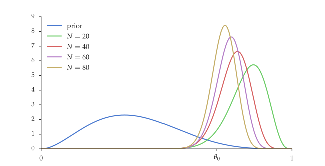
Figure 8.10:Evolution of the posterior from Beta prior
Point estimates are extracted from the posterior distribution based on some measure of central tendency, such as the mean, the median, or the mode of the posterior (i.e., the maximizer in the unimodal case).
The posterior we came up with in (8.44) belongs to the same parametric class as the prior. Priors where the parametric class is preserved under Bayesian updating for a specific likelihood function are called conjugate. Conjugacy makes application of Bayes’ law particularly simple.
In applications, the existence of a closed-form solution for the posterior is rare, and the integration over the parameter space in (8.41) has to be carried out numerically. The standard technique is Markov chain Monte Carlo. An exposition of the Metropolis–Hastings algorithm was given in Section 7.4.2. If you return to (7.38), you will notice how implementation of this algorithm only requires us to evaluate ratios of the posterior, which means that the integral term on the right-hand side of (8.41) cancels out. Because the integral can be very high dimensional, this often eliminates a huge amount of complexity.
Bayesian inference has experienced a surge of popularity in recent years. One reason is that in high dimensions, exploring the posterior via MCMC has proved to be more successful in practice than the numerical optimization required to obtain maximum likelihood estimates. Another is that Bayesian estimation provides a form of regularization that stabilizes and typically improves estimation of complex models. See Section 14.2.3. A third is that Bayesian estimation comes with an elegant, unified decision-theoretic approach to inference. Some discussion is given in Section 9.2.5.
8.4Further Reading¶
The ERM principle is a very general principle for solving statistical problems and producing estimators. For such a general method it is difficult to give a set of strong results showing that ERM produces good estimators. Indeed, there will be instances when ERM produces poor estimators, as discussed in Section 8.2.3. Having said that, some rather general consistency results have been obtained. Additional discussion can be found in Vapnik (2000).
There are many good treatments of Bayesian estimation available in the literature, including Geweke (2005), Geweke et al. (2011), and Kroese & Chan (2014).
Chernozhukov & Fernández-Val (2011) discuss quantile regression of the th quantile in cases where is close to zero or one.
8.5Exercises¶
8.5.1Solutions to Selected Exercises¶
Why not always try to infer itself? Although it’s true that when we know we can in principle recover any feature , we should also bear in mind the following general principle of inference with limited information: In solving a given problem, try to avoid first solving a more general problem as an intermediate step. Distributions are much more complicated objects than real numbers, so if we care only about the median of a distribution, say, it might be best to try to discover this single value directly rather than trying to infer the entire distribution first.
See, for example, §2.4 of Friedman et al. (2009).
The scare quotes on "unlikely" are just a reminder that our distribution is absolutely continuous and hence all individual outcomes have probability zero. When we say that an outcome is unlikely, we mean that there is little probability mass in the neighborhood of .
More precisely, if and only if almost everywhere. Densities are equal almost everywhere when the set of points at which they fail to be equal has Lebesgue measure zero.
- Benhabib, J., Bisin, A., & Zhu, S. (2015). The wealth distribution in Bewley economies with capital income risk. Journal of Economic Theory, 159, 489–515.
- Dudley, R. M. (2002). Real Analysis and Probability (2nd ed.). Cambridge, UK: Cambridge University Press.
- Manski, C. F. (1986). Analog estimation of econometric models. In R. F. Engle & D. McFadden (Eds.), Handbook of Econometrics (Vol. 4, pp. 2559–2582). Elsevier.
- Koenker, R., & Hallock, K. (2001). Quantile regression: an introduction. Journal of Economic Perspectives, 15(4), 43–56.
- Hansen, L. P. (2014). Nobel lecture: Uncertainty outside and inside economic models. Journal of Political Economy, 122(5), 945–987.
- Hansen, L. P., & Singleton, K. J. (1982). Generalized instrumental variables estimation of nonlinear rational expectations models. Econometrica, 50(5), 1269–1286.
- Vapnik, V. N. (2000). The Nature of Statistical Learning Theory (2nd ed.). New York: Springer.
- Geweke, J. (2005). Contemporary Bayesian Econometrics and Statistics. Hoboken, NJ: Wiley.
- Geweke, J., Koop, G., & Van Dijk, H. (2011). The Oxford Handbook of Bayesian Econometrics. Oxford: Oxford University Press.
- Kroese, D. P., & Chan, J. C. (2014). Statistical Modeling and Computation. New York: Springer.
- Chernozhukov, V., & Fernández-Val, I. (2011). Inference for extremal conditional quantile models, with an application to market and birthweight risks. Review of Economic Studies, 78(2), 559–589.
- Friedman, J., Hastie, T., & Tibshirani, R. (2009). The Elements of Statistical Learning (2nd ed.). New York: Springer.