In several sections of this book we touched on the topic of regularization (see, e.g., Section 8.2.1.2 and Section 8.2.3). A variety of statistical procedures and machine learning algorithms employ regularization (under different names) to improve out-of-sample fit. Good out-of-sample fit means generalization from observed data, which, as we’ve stressed before, is the key problem of statistics. This chapter introduces a number of methods that use regularization and discusses their statistical properties.
14.1Nonparametric Density Estimation
Nonparametric density estimation is an application of regularization to the problem of recovering distributions from data. It combines the data with a prior belief that probability mass most likely falls in places other than just the sample points observed so far. As well as being of interest from a theoretical perspective, nonparametric density estimation is used in a great variety of applied studies. We begin our analysis with a review of parametric density estimation and then proceed to nonparametric methods.
14.1.1Introduction
Suppose our data consist of IID observations from unknown distribution on . We assume throughout this section that is absolutely continuous. Our aim is to estimate the density of , denoted below by .
We know how to do this in a parametric setting. For example, let’s add the assumption that belongs to the class of normal densities on , so that the normal density for distribution . The MLEs of the parameters are and . Plugging these back into gives density estimate . Since and are consistent (see Section 9.2.4), the random density will be close to with high probability for large .
We can clarify convergence of the densities themselves if we extend the notion of consistency from vectors to densities. To extend consistency to densities we need a notion of global deviation between densities. Perhaps the most important measures of global distance are the distances. Let’s now define and discuss them.
For any -measurable function and , we set
where integration is over all of . If this expression is finite, then we write . For densities and on the distance between these densities is then defined as
The norm satisfies most of the properties of the norms we’ve met so far. For example, we have the triangle inequality
for all and . See, for example, theorem 5.1.5 of Dudley (2002).
Specializing to gives the distance, which sums over absolute deviation. Specializing to gives the popular distance, which is a variation of the distance we used in Section 5.2.2. See, in particular, (5.28), where distance between random variables is evaluated based on expected deviation.
The distance is popular largely because it’s so tractable, and because it’s similarity to Euclidean vector distance means that we have analogies for a variety of fundamental results on vector space. Nevertheless, the distance is arguably a better choice for studying deviation between densities. For example, the distance between densities is always well-defined (see ex. 14.4.1), which is essential if one hopes to provide universal consistency results.
The bound in (i) is called Pinsker’s inequality, while (ii) is called Scheffé’s identity. Scheffé’s identity tells us that distance measures something that we directly care about: when deviation is small, so is the maximal deviation between probabilities assigned to events.[1]
In what follows, we will say that a sequence of random densities on is -consistent for a density on if
14.1.1.1Failure of Consistency
The risk with the parametric approach is that the parametric assumption is incorrect, in the sense that the parametric class doesn’t contain the density generating the data or any good approximation. If this is the case, a parametric approach is typically not consistent. More precisely, if we estimate with parametric class , then the deviation between our estimate and is bounded below by
This value will be zero only when can be attained as the limit of elements of .
14.1.2Kernel Density Estimation
Sometimes we can make good choices for parametric classes by using descriptive statistics or by appealing to some theory with sharp quantitative implications. At other times this is difficult. In such settings it is best to use a nonparametric approach that is consistent under weaker assumptions.
Let’s start with an intuitive discussion and then turn to theory. Suppose that we have IID data generated from unknown density on . To estimate using the data we will employ a kernel density estimator (KDE), which takes the form
Here is called the kernel function of the estimator, and is called the bandwidth. The kernel function is required to be a density on but is otherwise unrestricted. The bandwidth is any positive number. Exercise 14.4.4 asks you to confirm that is always a density.
To get a feeling for the estimate in (14.5), let’s look at a simple instance created from just three data points on . For we take the standard normal density. Since , the function is the sum of three individual functions, the th of which can be written as
This is times the density of a random variable. So the three functions are smooth bumps, each centered on one of the data points and with the degree of concentration around governed by . The top panel of figure 14.1 shows these three functions along with the data points for when . The black line is the pointwise sum of these functions, which is the density estimate . By construction, it is large near the data points and small away from data points.
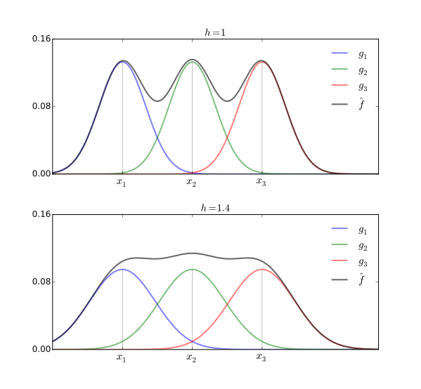
Figure 14.1:Nonparametric KDE, different bandwidths
The lower panel of figure 14.1 shows the same functions when the bandwidth is increased to . Each becomes more spread out, and the sum is smoother.
As discussed in more detail below, the role of the bandwidth is to add smoothing to the empirical distribution, so we can generalize from a finite sample. But what is the right amount of smoothing? Figure 14.2 illustrates the trade-off associated with smoothing. The shaded distribution is the density , which we imagine to be unknown. 40 observations are drawn from this distribution and represented as dots. The black line in each panel is the KDE built from these observations. The kernel is the standard normal density again, while the bandwidth varies across the panels.
As the bandwidth goes to zero, the kernel density becomes similar to the empirical distribution, with all probability mass in very small regions around the sample points. Hence, when we use a very small bandwidth , we make the mistake of treating the empirical distribution as the true distribution. This is overfitting. At the same time, excessive smoothing adds too much bias, hiding the features of the true distribution.[2]
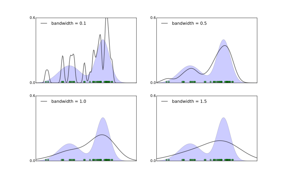
Figure 14.2:Effect of changing the bandwidth
The optimal bandwidth in terms of minimizing deviation depends on the unknown density . For example, if is smooth, then a relatively large bandwidth should be used. Of course is unknown. As such there are two standard approaches. One is to make assumptions on and choose the bandwidth accordingly. Another is to use cross-validation. For a review of both procedures see Scott (2015). We’ll say more about cross-validation in the context of ridge regression below.
14.1.3Theory
A natural way to study kernel density estimates is via the notion of convolutions. The convolution of an arbitrary distribution and a density on is the density on defined by
We already encountered this concept in the discrete case in exercise 5.4.10, where you were asked to prove a version of
We will be particularly interested in a certain class of convolutions, induced by densities of the form
where is any density and is a parameter. The density in (14.8) is the density of when is a random vector on with density . (See ex. 14.4.6.)
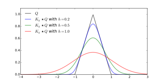
Figure 14.3:Smoothing induced by convolutions
Note how in figure 14.3 the distribution of is close to when is near zero. This makes sense, since is the distribution of where is drawn from and is standard normal. As we take , the distribution of converges to the distribution of . In fact this is always true:
For a proof, see theorem 9.1 of Devroye & Lugosi (2001).
14.1.3.1Convolution and KDEs
Let be a positive number and let be as defined in (14.8). Using this notation, we can rewrite the KDE in (14.5) as . Letting denote the empirical distribution of the sample and recalling the expression for integrals with respect to , we can also write this as , or, more simply,
This equation says something interesting. In Section 8.2.1.2 we first tried to estimate the density by a naive application of the sample analogue principle. The method failed. In (14.9) we have an alternative method that employs smoothing, or regularization. We apply the "smoothing operator" in addition to replacing the target distribution with the empirical distribution. As the next section shows, this method can be successful under very mild assumptions.
14.1.3.2Consistency
It can be proved that, for any density and kernel , the nonparametric kernel density estimator is -consistent for . See theorem 9.2 of Devroye & Lugosi (2001). The proof involves a large amount of measure-theoretic machinery. Here we’ll state and prove the corresponding result instead.
Let’s break this claim down into smaller pieces. For the remainder of this section, is the norm and . Using the expression for in (14.9) and the triangle inequality in (14.3), we have
The first term is called the estimation error, and the second is called the approximation error or bias. The first error is caused by the fact that we only observe the empirical distribution rather than the true distribution . The second error is caused by the smoothing we deliberately added to control the estimation error. (Compare with the error decomposition.)
The fact that in condition (ii) of theorem 14.1.1 means that we shrink the amount of smoothing as the sample size increases, thereby reducing the approximation error. The requirement ensures that smoothing is not reduced too quickly, allowing us to control estimation error.
One way to think about the relationship between inference and the sample is that, when viewed as a "generalized density" with all its mass on data points, the empirical distribution is too rough. To generalize we need to add smoothing. At the same time, the need for smoothing decreases as the sample size gets large.
14.1.4Commentary
In some fields of science, researchers have considerable knowledge about parametric classes and specific functional forms. For example, the theory of Brownian motion describes how the location of a tiny particle in liquid is approximately normally distributed. Thus the underlying theory provides an exact parametric class. In this kind of setting the parametric approach excels. It allows us to generalize by combining data with information we have on functional forms.
Unfortunately, the quantitative foundations of economics and other social sciences are looser and more prone to shifting over time. Econometricians usually come to the table with less knowledge of parametric classes and functional forms. These facts make nonparametric techniques attractive.
At the same time, nonparametric methods do not solve all our problems. The theoretical results presented above are purely asymptotic. Finite sample results are available, but it isn’t possible to obtain strong results in this direction without correspondingly strict assumptions on the target density. There is no uniform rate of convergence for all target densities (Devroye & Lugosi (2001), p. 85). This is because nonparametric methods have relatively little structure in the form of prior knowledge and hence require abundant data.
14.2Controlling Complexity
In the last section we discussed flexible estimation methods that perform well asymptotically. In this section we turn our attention to finite sample properties. A common thread will be ridge regression, which is a popular method of estimation in both econometrics and machine learning (see, e.g., Peysakhovich & Naecker (2015), Kim & Swanson (2014), or Varian (2014)). Ridge regression also connects to some deep ideas at the heart of finite sample theory, including complexity, prior knowledge and the bias–variance trade-off.
14.2.1Ridge Regression
Let’s start off in the classical OLS setting of Section 12.1.1, with assumptions 12.1.2–12.1.4 all in force. The usual OLS estimator is as given in (12.3). It can also be expressed as
As shown in Section 11.1.2, the OLS estimator minimizes the empirical risk under quadratic loss when the hypothesis space is the set of linear functions. Under our current assumptions, it is also unbiased for (theorem 12.1.1) and, by the Gauss–Markov theorem, it has the lowest variance among all linear unbiased estimators of (theorem 12.1.3).
While the Gauss–Markov theorem has historical importance, a more natural way to evaluate estimators is to consider their mean squared error, which tells us directly how much probability mass the estimator puts around the object it is trying to estimate (see Section 9.2.3). Recalling (9.9), the MSE of an estimator of is defined as
As exercise 14.4.8 asks you to show, the following representation is also valid:
This equation extends (9.10), and tells us that MSE is the sum of a variance and a bias term. Minimization of MSE involves a trade-off between these two terms. Typically, the optimal choice is not at either extreme: MSE is minimized when some amount of bias is admitted.
Applying this idea to the OLS setting, Hoerl & Kennard (1970) showed that there exists a biased linear estimator that has lower mean squared error than . The estimator is defined as the solution to the modified least squares problem
where is called the regularization parameter. In solving (14.14), we are minimizing the empirical risk plus a term that penalizes large values of . The effect is to “shrink” the solution relative to the unpenalized solution . Some calculus shows that the solution to (14.14) is
The estimator is called the ridge regression estimator. Note that
is the OLS estimator when and
is biased whenever (ex. 14.4.9).
The following result is proved in Hoerl & Kennard (1970).
The reduction in MSE over the least squares estimator occurs because, for some intermediate value of , the variance of falls by more than enough to offset the bias induced by regularization.
Note that, for suitable choice of , the ridge regression estimator outperforms even though all of the classical OLS assumptions are valid. At the same time, the right choice of is a nontrivial problem. This problem falls under the heading of model selection, which is the topic treated in the next few sections.
14.2.1.1Interpretation
The traditional view of ridge regression runs as follows: The standard OLS assumptions are treated as valid. There may, however, be instances where is almost singular due to strong correlation between regressors. In this case the process of inverting is numerically unstable. We can stabilize the inversion by adding some positive value of in (14.15).
Here’s another view: The standard OLS assumptions are implausible. Since our loss function is quadratic, we would ideally like to obtain the regression function but recovering this infinite dimensional object with a finite amount of data is ill-posed. We need to control the complexity of the candidate functions we use to approximate the regression function. The regularization term in ridge regression provides a means of managing complexity.
14.2.1.2Tikhonov Regularization
Let’s build some more intuition for the result in theorem 14.2.1 by running simulations. We’ll frame the simulations in a general setting, of which ridge regression is a special case.
We know that the least squares estimator is the solution to an overdetermined system of equations. There is an existing theory for solving ill-posed linear systems in high dimensions. The basic idea is that any attempt to back out or infer a complex object by solving a system about which we have limited information requires a degree of regularization.
To illustrate, suppose that
is an overdetermined system, where is with .
Due to measurement error, we only observe an approximation of .
is the (unobservable) least squares solution .
In the absence of additional information, a natural approach to approximating is to solve by least squares. An alternative, less obvious approach, is to minimize
for some small but positive . This second approach is called Tikhonov regularization. We are minimizing least squares plus a penalty term.
Let’s look at a simulation where is chosen stochastically but with a tendency towards multicollinearity. To aid clarity, we first set , and then set . By construction, is a solution to the system , and also the least squares solution.
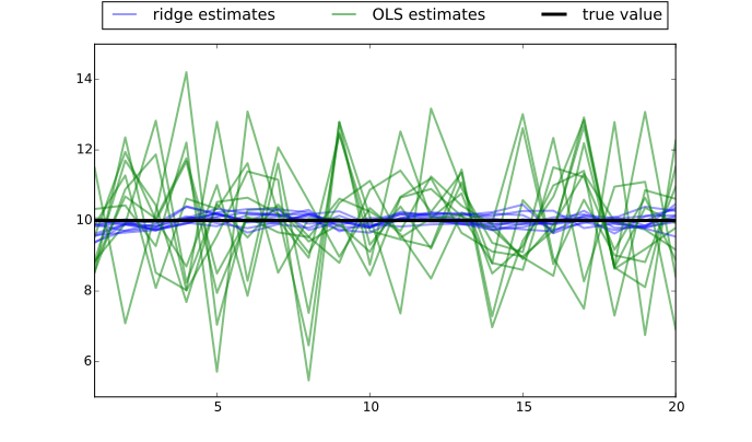
Figure 14.4:Effect of Tikhonov regularization,
Measurement of is corrupted with a Gaussian shock. In particular, is drawn from where is a small positive number. We then plot the OLS solution based on , which minimizes , and the regularized solution, which minimizes in (14.16). The former are plotted against their index in green, while the latter are plotted in blue. The true solution is plotted in black. The result is figure 14.4.
The figure shows 10 solutions each for the ordinary and regularized solutions, corresponding to 10 draws of . The regularized solutions are much closer to the true solution on average.
Note that this result is dependent on a reasonable choice for . If you experiment with the code on the text website, you will see that for very small values of , the regularized solutions are almost the same as the unregularized solutions. Conversely, very large values of pull the regularized solutions too close to the zero vector.
14.2.2Subset Selection and Ridge Regression
One problem frequently faced in regression problems is which variables to include. For example, if we are comparing crime rates across different cites, we can think of any number of variables that might be relevant (median wage, unemployment, police density, etc.). The same is true if we are trying to model credit default rates for some group of individuals, or educational attainment across schools. A similar problem arises in time series models, where we want to know how many lags of the state variables to include. The general problem is known as subset selection, since we are trying to choose the right subset of all candidate regressors.
Further dimensions appear when we consider basis functions. Given a set of covariates , we have the option to map this into a larger vector using basis functions, as discussed in Section 11.2.1. For example, given a single covariate , we may consider mapping it into and regressing on . As we saw in figures 8.5–8.8, a good choice of is crucial. Choosing is another example of the subset selection problem because we are trying to decide whether to include the regressor for some given .
Subset selection is a version of the empirical risk minimization problem. Suppose that we have output and inputs , in the sense that contains candidate regressors. If we want to include all regressors, then we can minimize empirical risk over in (11.4), the hypothesis space of linear functions from to . If we wish to exclude some subset of regressors, we can set to be the set of indices of the regressors we want to exclude and regress on the remainder, which is equivalent to minimizing the empirical risk over the hypothesis space
We are back to the problem of choosing a suitable hypothesis space over which to minimize empirical risk.
The subset selection problem has been tackled by many researchers. Well-known approaches include the Akaike Information Criterion (AIC), the Bayesian Information Criterion (BIC), and Mallow’s statistic. For example, Mallow’s statistic consists of two terms, one increasing in the size of the empirical risk, and the other increasing in , the size of the subset selected. The objective is to minimize the statistic, which involves trading off poor fit (large empirical risk) against excess complexity of the hypothesis space (large ).
One of the problems with subset selection is that regressors means subsets to step through.[3] To avoid this computational problem, one alternative is to use ridge regression. With ridge regression, the regularization term leads us to choose an estimate with smaller norm. What this means, in practice, is that the coefficients of less helpful regressors are driven towards zero, thereby “almost excluding” those regressors. While the model selection problem is not solved, it has been reduced to tuning a single parameter.
We can illustrate the idea by reconsidering the regression problem discussed in Section 8.2.3. Figure 8.5–Figure 8.8 showed the fit we obtained by minimizing empirical risk over larger and larger hypothesis spaces. The hypothesis spaces were the sets of degree polynomials for different values of . For each we minimized the empirical risk over , which translates into solving
As discussed above, choosing the right is isomorphic to subset selection, since we are deciding what powers of to include as regressors. Figure 8.4 showed that intermediate values of did best at minimizing risk.
We can do a similar thing using ridge regression. First, let’s take as our hypothesis space. This space is certainly large enough to provide a good fit to the data, but with empirical risk minimization the result is overfitting (see figure 8.8). Here, instead of using empirical risk minimization, we solve the regularized problem
for different values of . The data used here are exactly the same data used in the original figures 8.5–8.8 from Section 8.2.3. The solution for each we denote by , which is the ridge regression estimator, and the resulting prediction function we denote by , so that .
The function is plotted in red for increasingly larger values of over figures 14.5–14.7. The black line is the risk-minimizing function. In figure 14.5, the value of is too small to impose any real restriction, and the procedure overfits. In figure 14.6, the value of is larger and the fit is good. In figure 14.7 the value of is too large and the estimate is poor.
As in Section 8.2.3, we can compute the risk of each function , since we know the underlying model (see (8.25)). The risk is plotted against in figure 14.8. The -axis is on log-scale. The risk is smallest for small but nonzero values of .
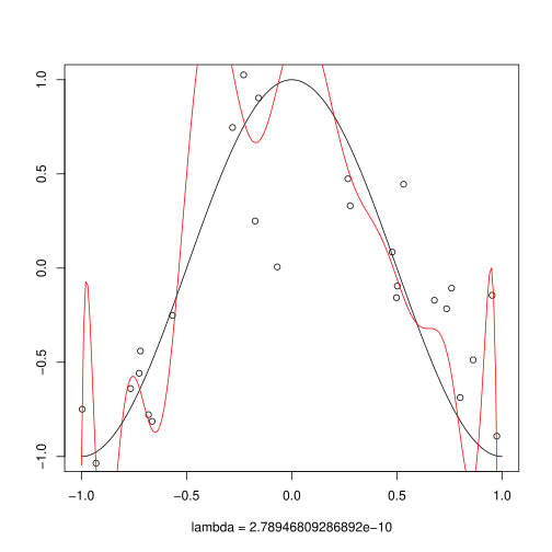
Figure 14.5:Fitted polynomial,
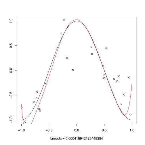
Figure 14.6:Fitted polynomial,
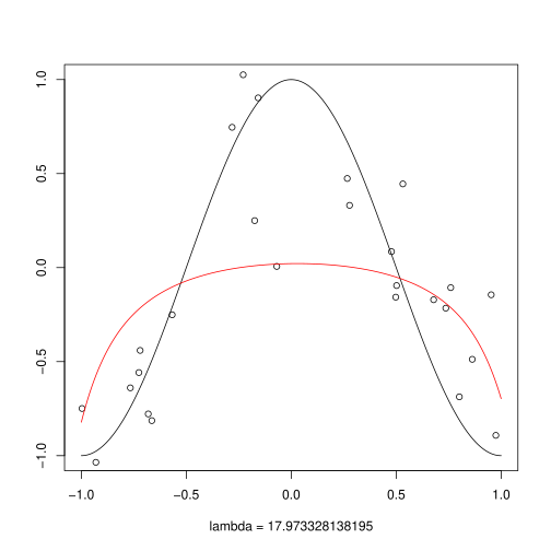
Figure 14.7:Fitted polynomial,
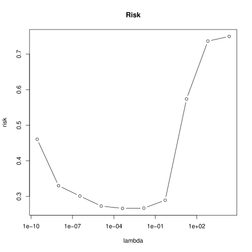
Figure 14.8:Risk of plotted against
14.2.3Bayesian Methods and Regularization
The ideal case with model selection is that we have clear guidance from economic theory on which regressors to include, which functional forms to use, which values of our regularization parameter to choose, and so on. If theory or prior knowledge provides this information, then every effort should be made to exploit it. One technique for injecting prior information into statistical estimation is via Bayesian analysis. Let’s now look at Bayesian linear regression and how it compares to ridge regression.
Suppose that our regression data take the linear form . To simplify the presentation we will assume that is nonrandom. (Taking to be random leads to the same conclusions but with a longer derivation). As before, is random and unobservable. The new feature provided by the Bayesian perspective is that we take to be random and unobservable as well. In addition we are assumed to have subjective prior beliefs regarding likely values for these variates, expressed in the form of probability distributions. Here we take the priors to be and .
Given our model , our prior on implies that the density of given is . In generic notation, we can write our distributions as
Applying Bayes’ law (see (5.25)) to the pair , we obtain
The left-hand side is the posterior density of given the data , and represents our new beliefs updated from the prior on the basis of the data .
One way to summarize the information contained in the posterior is by examining its maximum value. The maximizer of the posterior is called the maximum a posteriori (MAP) probability estimate. Taking logs of (14.18) and dropping the term that does not contain , it can be expressed as
Inserting our functional forms into (14.17), dropping constant terms and multiplying by , we obtain the expression
This is precisely the penalized least squares problem (14.14), where the regularization parameter is equal to . In view of (14.15), the solution is
Thus Bayesian estimation provides a principled derivation of the penalized objective function from ridge regression. Bayesian analysis provides the same effect as Tikhonov regularization, but now regularization arises out of combining prior knowledge with the data. Moreover, at least in principle, the value is part of our prior knowledge, and hence there is no model selection problem.
In practice, one could of course question the assertion that we have so much prior knowledge that the regularization parameter is pinned down. If such knowledge is lacking, then we are back at the model selection problem. In the next section we forgo the assumption that this strong prior knowledge is available, and consider a more automated approach to choosing .
14.2.4Cross-Validation
A natural way to think about model selection is to think about minimizing risk. Recall that, given loss function and a system producing input–output pairs with joint distribution , the prediction risk of a function is the expected loss
that occurs when we use to predict . Now suppose that we observe IID input–output pairs . Given a selection of models, we would like to find the one that takes this data set and returns a predictor such that has lower prediction risk than the predictors returned by the other models.
We have to be precise in defining risk because, if we define it as , then we are taking expectation over all randomness, including that in , which depends on the data set . What we want to do now is take the data set as given, and see how well we can do in terms of predicting new values as evaluated by expected loss. Hence we define the prediction risk of to be the expected loss taking (and hence ) as given:
If we have a collection of models indexed by , and is the predictor produced by fitting model with data , then we would like to find the model such that
The obvious problem with this idea is that risk is unobservable. If we knew the joint distribution then we could calculate it; but then again, if we knew there would be no need to estimate anything in the first place.
Looking at this problem, you might have the following idea: Although we don’t know , we do have the data , which consists of IID draws from . From the law of large numbers, we know that expectations can be approximated by averages over IID draws, so we could approximate by
where the pairs are from the data set .
However, this is just the empirical risk, and the empirical risk is a highly biased estimator of the risk. This point was discussed extensively in Section 8.2.3. See, in particular, figure 8.4. The point that figure made was that complex models tend to overfit, producing low empirical risk, but high risk. In essence, the problem is that we are using the data twice, for conflicting objectives. First, we are using it to fit the model, producing . Second, we are using it to evaluate the predictive ability of on new observations.
So what we really need is fresh data. New data will tell us how performs out-of-sample. If we had new observations , then we could estimate the risk by
Of course, this isn’t a genuine solution because we don’t have any new data in general. One way to work around this problem is to take and split it into two disjoint subsets, called the training set and the validation set. The training set is used to fit and the validation set is used to estimate the risk of . We then repeat this for all models and choose the one with lowest estimated risk.
Since data are scarce, a more common procedure is cross-validation, which attempts to use the whole data set for both fitting the model and estimating the risk. To illustrate the idea, suppose that we partition the data set into two subsets and . First, we use as the training set and as the validation set. Next we use as the training set, and as the validation set. The estimate of the risk is the average of the estimates of the risk produced in these two steps.
Of course, we could divide the data into more than two sets. The extreme is to partition the data into subsets. This procedure is called leave-one-out cross-validation. Letting , the data set with just the th data point omitted, the leave-one-out cross validation algorithm can be expressed as follows:
for do
fit using data
set
end
return the risk estimate
At each step inside the loop, we fit the model using all but the th data point, and then predict the th data point using the fitted model. The prediction quality is evaluated in terms of loss. Repeating this times, we produce an estimate of the risk using average loss. On an intuitive level, the procedure is attractive because we are using the available data intensively but still evaluating based on out-of-sample error.
In terms of model selection, the idea is to run each model through the cross-validation procedure, and then select the one that produces the lowest value of , the estimated risk. Let’s illustrate this idea, by considering again the ridge regression procedure used in Section 14.2.2. In this problem the set of models is indexed by , the regularization parameter in the ridge regression. The data set is the set of points shown in figures 14.5–14.7. For each , the fitted function is
Recall here that with fixed at 14, so we are fitting a polynomial of degree 14 to the data by minimizing regularized least squares error. The amount of regularization is increasing in . The resulting functions were shown for different values of in figures 14.5–14.7. Intermediate values of produced the best fit in terms of minimizing risk (see figures 14.6 and 14.8).
In that discussion, we used the fact that we knew the underlying model to evaluate the risk, and hence the values of that produce low risk (figure 14.8). In real estimation problems, risk is unobservable, and we need to choose on the basis of the data alone (assuming we don’t have prior knowledge, as in the Bayesian case—see Section 14.2.3). Let’s see how a data-based procedure such as cross-validation performs in terms of selecting a good value of .
In this experiment, for each in the grid exp(seq(-22, 10, length=10)) we perform leave-one-out cross-validation. The fit at each step within the loop is via ridge regression, omitting the th data point, and the resulting polynomial is used to predict from . The prediction error is measured by squared loss. In other words, for each in the grid, we use the following algorithm to estimate the risk:
for do
set
set
end
return
The value of producing the smallest estimated risk is around 0.015. This is in fact very close to the value that minimizes the actual risk (see figure 14.8). The associated function is plotted in red in figure 14.9, and indeed the fit is close. In this instance, our fully automated procedure is successful.
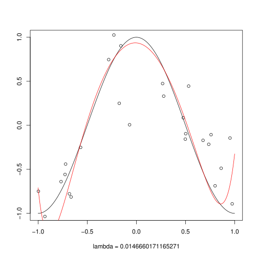
Figure 14.9:Fitted polynomial,
14.3Further Reading
Textbook treatments of nonparametric methods in econometrics can be found in Pagan & Ullah (1999), Li & Racine (2006), Ullah (1989), Henderson & Parmeter (2015) and Hansen (2015). Bosq (1996) covers nonparametrics for time series models. Recent studies in the econometrics literature using nonparametric or semiparametric methods include Chen & Hong (2012), Jeong et al. (2012), Henderson et al. (2012), Christensen (2014), Canay et al. (2013), Su & Ullah (2013), Bajari et al. (2013), Newey (2013), Hansen (2014), Mastromarco & Simar (2015), Hickman & Hubbard (2015), Matzkin (2015), Bhattacharya (2015), and Du & Escanciano (2015). A beautiful overview of nonparametrics and the method of sieves can be found in Geman & Hwang (1982).
Good discussions of ridge regression and cross-validation can be found in Friedman et al. (2009) and Abu-Mostafa et al. (2012). One alternative to ridge regression is the LASSO method (Tibshirani (1996)), where the term in (14.14) is replaced with an absolute deviation penalty . Also related is penalized maximum likelihood estimation. A recent application can be found in Gentzkow et al. (2015).
An important contribution to the literature on subset selection is the least angle regression of Efron et al. (2004). A discussion of this method in relation to other subset techniques can be found in Hesterberg et al. (2008).
Recent papers treating regularization and related topics within the econometrics literature include Florens (2003), Carrasco et al. (2007), Chen & Reiss (2011), Florens & Simoni (2014), Darolles et al. (2011), Hoderlein & Holzmann (2011), Horowitz (2014), Hautsch et al. (2012), Li et al. (2015), Lunde et al. (n.d.), Chernozhukov et al. (2015), and Ando & Bai (n.d.).
Regarding implementations, one powerful and increasingly popular package for Bayesian learning is Stan. See http://mc-stan.org/. A popular and high-quality routine for cross validation in the context of ridge regression can be found in the sklearn.linear_model.RidgeCV method in Python’s scikit-learn package.
14.4Exercises
14.4.1Solutions to Selected Exercises
For a proof, see p. 39 of Devroye & Lugosi (2001).
Figure 14.2 is produced using
scikit-learn. In R, KDEs can be constructed from thedensityfunction. Try, for example,plot(density(runif(200))).Remember Martin (1997) and his two million growth regressions?
Hint: It is a basic property of integration that pointwise implies .
Hint: Use fact 14.1.2 and exercise 8.5.9.
Hint: Try a change-of-variables argument.
- Dudley, R. M. (2002). Real Analysis and Probability (2nd ed.). Cambridge, UK: Cambridge University Press.
- Scott, D. W. (2015). Multivariate Density Estimation: Theory, Practice, and Visualization (2nd ed.). Hoboken, NJ: Wiley.
- Devroye, L., & Lugosi, G. (2001). Combinatorial Methods in Density Estimation. New York: Springer.
- Peysakhovich, A., & Naecker, J. (2015). Machine learning and behavioral economics: evaluating models of choice under risk and ambiguity [Techreport].
- Kim, H. H., & Swanson, N. R. (2014). Forecasting financial and macroeconomic variables using data reduction methods: New empirical evidence. Journal of Econometrics, 178, 352–367.
- Varian, H. R. (2014). Big data: New tricks for econometrics. The Journal of Economic Perspectives, 28, 3–27.
- Hoerl, A. E., & Kennard, R. W. (1970). Ridge regression: biased estimation for non\-orthogonal problems. Technometrics, 12(1), 55–67.
- Pagan, A., & Ullah, A. (1999). Nonparametric Econometrics. Cambridge, UK: Cambridge University Press.
- Li, Q., & Racine, J. S. (2006). Nonparametric Econometrics: Theory and Practice. Princeton: Princeton University Press.
- Ullah, A. (1989). Semiparametric and Nonparametric Econometrics. Heidelberg: Physica.
- Henderson, D. J., & Parmeter, C. F. (2015). Applied Nonparametric Econometrics. Cambridge, UK: Cambridge University Press.
- Hansen, B. E. (2015). Econometrics. Textbook in preparation. http://www.ssc.wisc%20edu/~bhansen/econometrics
- Bosq, D. (1996). Nonparametric Statistics for Stochastic Processes: Estimation and Prediction (Vol. 110). New York: Springer.
- Chen, B., & Hong, Y. (2012). Testing for smooth structural changes in time series models via nonparametric regression. Econometrica, 80(3), 1157–1183.
- Jeong, K., Härdle, W. K., & Song, S. (2012). A consistent nonparametric test for causality in quantile. Econometric Theory, 28(04), 861–887.