13 Large Samples and Dependence

With IID data, the joint distribution of the sample is pinned down by the common marginal of the observations. The statistical learning problem becomes one of learning the marginal. With dependent data the joint distribution is more complex. The fundamental statistical problem has to be extended as follows:

Let’s look at how we might tackle this problem, starting with least squares.

13.1Large Sample Least Squares¶

Our treatment of least squares in this chapter permits dependent data but at the same time requires that the sample size is large. Large samples allow us to drop some of the strict parametric assumptions on the error term we made when we considered finite sample inference (see, e.g., assumption 12.1.5). In this sense, the theory developed below is also useful for cross-sectional environments with no correlation between observations.

13.1.1Setup and Assumptions¶

Let’s go back to the linear model assumption of chapter 12. That is, we assume that our data $(y_1, \boldx_1), \ldots, (y_T, \boldx_T)$ are generated by the linear model

where $\boldbeta$ is a $K$-vector of unknown coefficients, and $u_t$ is an unobservable shock. Observations are indexed by $t$ rather than $n$ to remind us that observations are dependent. The sample size will be denoted by $T$.

We let $\boldy$ be the $T \times 1$ vector of observed outputs, so that $y_t$ is the $t$th element of $\boldy$, and $\boldu$ be the vector of shocks, so that $u_t$ is the $t$th element of $\boldu$. We let $\boldX$ be the $T \times K$ matrix $\boldX := (x_{tk})$, where $1 \leq t \leq T$ and $1 \leq k \leq K$.

We will estimate the parameter vector $\boldbeta$ via least squares. The OLS estimate is therefore unchanged at

(Recall (11.17).) The expression for the sampling error in (12.4) can be expanded into sums to obtain

In this section we drop the exogeneity assumption $\EE[\boldu \given \boldX] = \boldzero$ (assumption 12.1.3) because it excludes too many dynamic models. For example, we know from Section 12.2.2 that exogeneity fails when we try to estimate the simple AR(1) model $y_{t+1} = \beta y_t + u_{t+1}$ by setting $x_t = y_{t-1}$, thereby producing the regression model

For this specification of (13.1), the regressor is correlated with lagged values of the shock.

The full column rank condition is the same as assumption 11.1.1 and ensures that expressions like the matrix inverse in (13.2) make sense. Condition (i) is borrowed from the identical condition given in (11.10) and ensures that the limit in (13.2) exists. Condition (ii) gives convergence.

Assumption 13.1.2 permits dependence between current shocks and future regressors. This is desirable in a time series setting, since current shocks usually feed into future state variables.

One consequence of assumption 13.1.2 is that

The proof is an exercise (ex. 13.4.4).

A useful implication of assumptions 13.1.1 and 13.1.2 is that linear functions of $\{\boldx_t u_t\}$ form a martingale difference sequence (MDS). This will allow us to apply the sample path results in theorem 7.3.1.

13.1.2Consistency¶

Under the conditions of Section 13.1.1, the OLS estimator $\hboldbeta_T$ is consistent for $\boldbeta$:

13.1.2.1Consistency of $\hat \sigma^2_T$¶

In (12.5) we estimated the error variance $\sigma^2$ using $\hat \sigma^2 := \rss / (N - K)$, with $N$ being the sample size. Here the sample size is $T$, and since $T$ is assumed to be large relative to $K$, we have $1/(T-K) \approx 1/T$. Hence in this chapter we set $\hat \sigma^2_T = \rss / T$ instead. (None of the following theory is affected if we use $\rss / (T-K)$, however.)

13.1.3Asymptotic Normality of $\hboldbeta$¶

Next we show that $\sqrt{T} (\hboldbeta_T - \boldbeta)$ is asymptotically normal. From this information we can develop asymptotic tests and confidence intervals.

13.1.4Large Sample Tests¶

In Section 12.1.4.1 we considered the problem of testing a hypothesis about an individual coefficient $\beta_k$. Let’s consider this problem again in the large sample setting. The hypothesis to be tested is

In Section 12.1.4.1 we showed that if the error terms are normally distributed, then the expression $(\hat \beta_k - \beta_k) / \se(\hat \beta_k)$ is $t$-distributed with $N-K$ degrees of freedom. In the large sample case, we can use the CLT to show that the same statistic is asymptotically normal.^[1] The next theorem gives details.

In the theorem, $\hat \sigma_T$ is as defined in (13.8) and $v_k (\boldX)$ is the $(k,k)$th element of $(\boldX^\T \boldX)^{-1}$.

13.2MLE for Markov Processes¶

Let’s now turn to nonlinear estimation in a time series setting, using maximum likelihood. We will cover just the foundations of building and maximizing the likelihood.

13.2.1The Likelihood Function¶

If we have IID observations from some common density, then, as we saw in Section 8.3.1, the likelihood function for that data is the product of the marginals evaluated at the sample. If, instead, the data contains dependence, the likelihood is more complex.

One intermediate case is Markov processes, the joint distribution of which was given in (7.17). Suppose that the transition density $p_{\boldtheta}$ depends on some unknown parameter vector $\boldtheta \in \Theta$. Suppose further that the process has a unique stationary density $\pi_{\infty}^{\boldtheta}$ for all $\boldtheta$, and that $\boldx_1$ is a draw from this stationary density. Then the log-likelihood function is given by

In practice, it is usual to drop the first term in this expression, particularly when the data size is large, since the influence of a single element is likely to be negligible. In addition, even though the stationary density is formally defined by (7.19), for many processes, there is no known analytical expression for this density.^[2] Here we’ll follow this convention and, abusing notation slightly, write

13.2.1.1Example: The ARCH Case¶

Let’s look at a relatively simple case: the ARCH model from (7.5). By (13.17), the log-likelihood function is

Rearranging, dropping terms that don’t depend on $a$ or $b$, and multiplying by 2 (an increasing transformation), we can rewrite this (abusing notation again) as

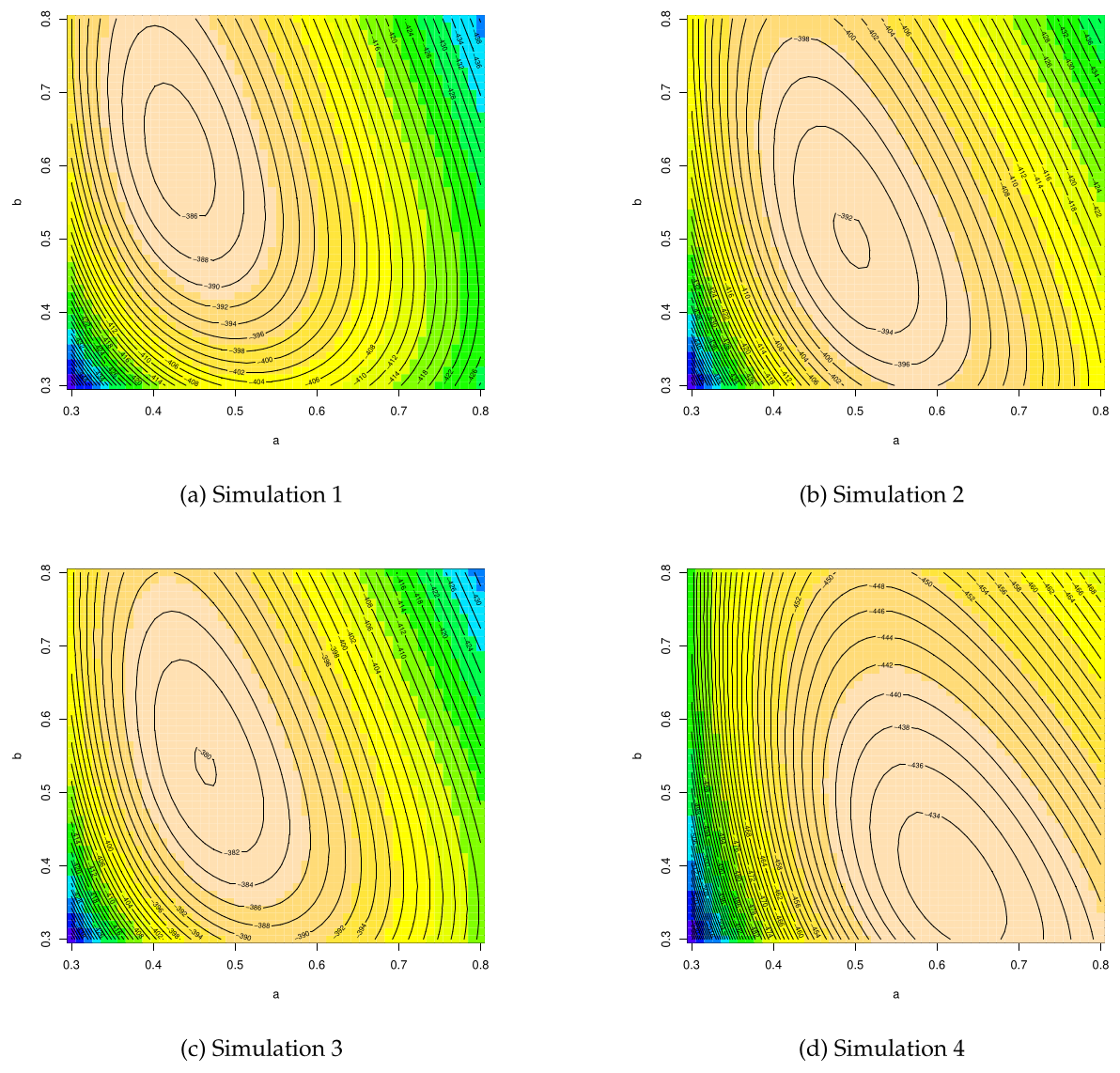
Let’s run some simulations to see what this function looks like. In the simulations we will set $T=500$ and $a=b=0.5$. Thus, we imagine the situation where, unbeknown to us, the true parameter values are $a=b=0.5$, and we observe a time series $x_1,\ldots,x_{500}$ generated by these parameters. In order to estimate $a$ and $b$, we form the likelihood function (13.19), and obtain the MLEs $\hat a$ and $\hat b$ as the vector $(\hat a, \hat b)$ that maximizes $\ell(a,b)$.

Four different simulations of $\ell$ are given in figure 13.1. In each figure, a separate data set $x_1,\ldots,x_{500}$ is generated using the true parameter values $a=b=0.5$ and the function $\ell$ in (13.19) is then plotted using contour lines and a color map. Lighter colors refer to larger values. The horizontal axis is $a$ values, and the vertical axis is $b$ values. The code for producing one of these figures (modulo randomness) is given in listing 11. The function arch_like(theta, data) represents $\ell$ in (13.19), with theta corresponding to $(a,b)$ and data corresponding to the time series $x_1,\ldots,x_T$.

In each of the four simulations, a rough guess of the MLEs can be obtained just by looking for maximizers in the figures. For example, in simulation (a), the MLEs look to be around $\hat a = 0.44$ and $\hat b = 0.61$. To get more accurate estimates, we can use some form of analytical or numerical optimization. For this problem we don’t have any analytical expressions for the MLEs because setting the two partial derivatives of $\ell$ in (13.19) to zero does not yield neat expressions for $\hat a$ and $\hat b$. However, there are many numerical routines we can use to obtain the MLEs for a given data set.

The simplest approach is to use one of R’s inbuilt optimization routines. For example, given the definition of arch_like in listing 11 and a sequence of observations $x_1,\ldots,x_T$ stored in a vector xdata, the function arch_like can be optimized numerically via the commands

start_theta <- c(0.65, 0.35)  # An initial guess of (a,b)
neg_like <- function(theta) {
    return(-arch_like(theta, xdata))  # xdata is the data
}
opt <- optim(start_theta, neg_like, method="BFGS")

Here optim is an built-in R function for numerical optimization of multivariate functions. Most built-in functions perform minimization rather than maximization and optim is no exception. For this reason the function that we pass to optim is neg_like, which is $-1$ times $\ell$. The first argument to optim is a vector of starting values (a guess of the MLEs). The last argument tells optim to use the BFGS routine, which is variation on the Newton–Raphson algorithm. The return value of optim is a list, and the approximate minimizing vector is one element of this list (called par).

In this particular setup, for most realizations of the data and starting values, you will find that the algorithm converges to a good approximation to the global optimizer. However, there’s no guarantee that it will. In case of problems, it’s useful to know how these kinds of algorithms work, and how to code up simple implementations on your own. The next section will get you started.

arch_like <- function(theta, data) {
    Y <- data[-1]             #  All but first element
    X <- data[-length(data)]  #  All but last element
    Z <- theta[1] + theta[2] * X^2
    return(-sum(log(Z) + Y^2 / Z))
} 

sim_data <- function(a, b, n=500) {
    x <- numeric(n)
    x[1] = 0
    w = rnorm(n)
    for (t in 1:(n-1)) {
        x[t+1] = sqrt(a + b * x[t]^2) * w[t]
    }
    return(x)
}

xdata <- sim_data(0.5, 0.5)  #  True parameters

K <- 50
a <- seq(0.3, 0.8, length=K)
b <- seq(0.3, 0.8, length=K)
M <- matrix(nrow=K, ncol=K)
for (i in 1:K) {
    for (j in 1:K) {
        theta <- c(a[i], b[j])
        M[i,j] <- arch_like(theta, xdata)
    }
}
image(a, b, M, col=topo.colors(12))
contour(a, b, M, nlevels=40, add=T)

13.2.2The Newton–Raphson Algorithm¶

The Newton–Raphson algorithm is a root-finding algorithm. In other words, given a function $g \colon \RR \to \RR$, the algorithm searches for points $\bar s \in \RR$ such that $g(\bar s) = 0$. Any root-finding algorithm can be used to optimize differentiable functions because, for differentiable functions, interior optimizers are always roots of the objective function’s first derivative.

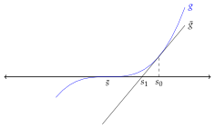
To describe the algorithm, let’s begin with the root-finding problem and then specialize to optimization. To begin, let $g \colon \RR \to \RR$, and let $s_0$ be some initial point in $\RR$ that we think (hope) is somewhere near a root. We don’t know how to jump from $s_0$ straight to a root of $g$ (otherwise, there would be no problem to solve), but what we can do is move to the root of the function that forms the tangent line to $g$ at $s_0$. In other words, we replace $g$ with its linear approximation around $s_0$, which is given by

and solve for the root of $\tilde g$. This point is represented as $s_1$ in figure 13.2, and the value is easily seen to be $s_1 := s_0 - g(s_0)/g'(s_0)$. The point $s_1$ is taken as our next guess of the root, and the procedure is repeated, taking the tangent of $g$ at $s_1$, solving for the root, and so on. This generates a sequence of points $\{s_k\}$ satisfying

There are various results telling us that when $g$ is suitably well-behaved and $s_0$ is sufficiently close to a given root $\bar s$, then sequence $\{s_k\}$ will converge to $\bar s$.^[3]

To move from general root-finding to the specific problem of optimization, suppose now that $g \colon \RR \to \RR$ is a twice differentiable function we wish to maximize. We know that if $s^*$ is a maximizer of $g$, then $g'(s^*) = 0$. Hence it is natural to begin our search for maximizers by looking for roots to this equation. This can be done by applying the Newton–Raphson algorithm to $g'$, which yields the sequence

We can extend this algorithm to the multivariate case as well. Let’s suppose that $g$ is a function of two arguments. In particular, suppose that $g$ is twice differentiable and $g \colon \RR^2 \to \RR$. The gradient vector and Hessian of $g$ at $(x,y) \in \RR^2$ are defined as

Here $g'_i$ is the first partial of $g$ with respect to its $i$th argument, $g''_{ij}$ is the second cross-partial, and so on.

By analogy with (13.20), the Newton–Raphson algorithm for this two dimensional case is the algorithm that generates the sequence $\{(x_k, y_k)\}$ defined by

from some initial guess $(x_0, y_0)$.^[4]

For the sake of the exercise, let’s apply this to maximization of (13.19). Let $z_t$ be as defined in (13.19). The first partials are then

while the second partials are

The cross-partial is

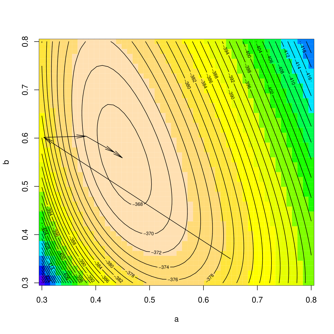
From these expressions we can form the gradient vector and the Hessian, pick an initial guess, and iterate according to (13.21). Figure 13.3 shows four iterations of this procedure, starting from $(a_0, b_0) = (0.65, 0.35)$.^[5] In this case the convergence is quick, and we are already close to the global optimum.

Replication of this figure (modulo randomness) is left as an exercise.

13.3Further Reading¶

Suitable topics for study after reading this chapter include GARCH models, hidden Markov models, Markov switching models, stochastic volatility models, factor models, and cointegration. High-quality textbook treatments of these and other topics in time series econometrics include Martin et al. (2012) and Hamilton (1994). Useful chapters on time series econometrics can be found in Hansen (2015) and Hayashi (2000). For a recent survey, see Diebold et al. (2009). For financial applications, see, for example, Ruppert (2011).

13.4Exercises¶

Incidentally, (13.23) can be used to test the null hypothesis that $\boldtheta = \boldtheta_0$. Under the null hypothesis, we have

Fixing $\alpha$ and letting $c$ be the $1-\alpha$ quantile of the $\chi^2(K)$ distribution, we reject the null if $T \| \hat \boldD_T (\hat \boldtheta_T - \boldtheta_0) \|^2 > c$. This test is asymptotically of size $\alpha$.

13.4.1Solutions to Selected Exercises¶