National Graduate Institute for Policy Studies (GRIPS)
When the concept of estimators was first introduced in Section 8.1.2 we mentioned that there is nothing in the definition that guarantees—or even alludes to—good performance. Let’s now start to think about evaluating estimators.
Our first step is to view estimators as random entities dependent on the data, and to consider their distributions under different specifications of the data-generating process. The notation below follows that set out in Section 8.1.1.
By definition, a statistic T is a B-measurable transformation of the sample space ZD into some feature space S. As a function of the sample zD=(z1,…,zN), it can be viewed as a random element mapping outcomes in the underlying space Ω to S via
ω↦T[zD(ω)]∈S
Here "random element" stands for either a random vector (or scalar), or something more general, such as the random distribution P^N, or a density estimate, which is a random function of the sample.
The idea that estimators are random can be counterintuitive. When we begin to study econometrics, we tend to think of data as fixed numbers determined by some prior historical outcome and statistics as deterministic functions of these numbers. Hence we only observe one value of any particular statistic—one sample mean, one sample variance, and so on. However, if we want to build a theory of estimators, then we need to consider their performance prior to observing the data. Each data set is viewed as a random draw from some unknown distribution. We seek estimators that perform well in the face of this uncertainty.
Once we agree that estimators are random, we know they must have distributions. These distributions determine how effective an estimator is at estimating the intended feature. Let’s now turn to investigating these distributions.
Suppose that T is a statistic mapping data zD into S. As just discussed, T(zD) is a random element taking values in S. Its distribution L(T) on S can be expressed as
L(T) is called the sampling distribution of T. Continuing to write PD for the joint distribution of the sample zD, we can also define the sampling distribution as
L(T)(B)=PD{s∈ZD:T(s)∈B}
or even PD∘T−1 if you like that kind of notation. Note that the sampling distribution of T is fully determined by
the statistic T that maps data to feature space,
the joint distribution PD of the data.
Since PD is unknown, the sampling distribution is likewise unknown. It can, however, be estimated, as we’ll see below.
Mathematically, there is no difference between the "sampling distribution of T" and the "distribution of T." Nonetheless, the terminology is standard.
Sampling distributions are often complicated. Sometimes the best we can do is obtain the sampling distribution of some transformation of an estimator.
To see why (9.4) holds, recall from example 2.2.3 that if S:=span{1} and P=projS, then the residual projection satisfies Mx=x−xˉ1. Hence
NsN2=n=1∑N(xn−xˉN)2=∥Mx∥2
Since M1=0 (see fact 2.2.8) and M is idempotent and symmetric (fact 3.3.2), setting ξ:=σ−1(x−μ1) gives
To see that the right-hand side has distribution χ2(N−1), apply fact 3.3.4 to obtain traceM=N−1, followed by fact 5.1.19.
Many long and involved proofs of fact 9.1.1 can be found in the literature, but a simple and informative proof can be obtained from fact 5.1.13. See exercise 9.4.2 and its solution.
In the preceding examples we were able to obtain an analytical expression for the sampling distribution of our estimator (or a simple transformation of the estimator) from the underlying distribution of the data. In reality this case is the exception.
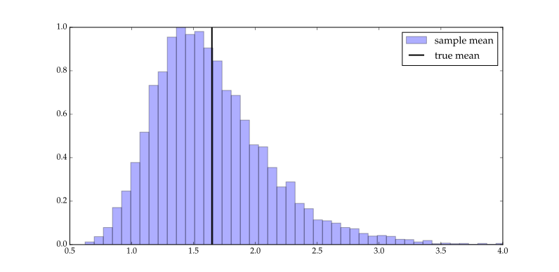
When no closed-form exists, we can still approximate the sampling distribution using simulation, conditional on a specification of the joint distribution of the data. For example, figure 9.1 shows a histogram approximation to L(xˉN) when N=20 and x1,…,xN is IID LN(0,1). The histogram is produced by generating 10,000 observations of xˉN. The loop that produced the observations is given in listing 5.
Figure 9.1:Sampling distribution of xˉN when N=20 and data are IID LN(0,1)
import numpy as np

N = 20
num_reps = 10000
xbar_outcomes = np.empty(num_reps)  # Allocate memory

for i in range(num_reps):
    x = np.exp(np.random.randn(N))  # Generate N iid lognormal RVs
    xbar_outcomes[i] = x.mean()
Listing 5:Generates 10,000 observations of the sample mean (Python)
The quality or performance of a given estimator is characterized by its sampling distribution. Let γ^ be an estimator of some feature γ based on a sample zD. What would be an ideal sampling distribution for γ^? The answer is obvious: a point mass that puts probability one on the single point γ.
This scenario rarely arises because our sample is random. So here’s a more realistic objective:
It is desirable that the sampling distribution of an estimator of γ concentrate most of its probability mass in a small neighborhood around γ, regardless of the joint distribution PD of the sample.
This statement considers only what is desirable, not what is possible. For example, if we look back at figure 9.1, we see that the sampling distribution of xˉN does not cluster tightly around the mean. (The feature γ that we are estimating is the mean of the LN(0,1) distribution, which is represented by the vertical black line.) But this is not unexpected, since the sample size is only 20. We simply don’t have enough information to estimate the feature precisely.
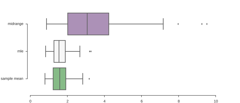
Nonetheless, these ideas give us a way to start comparing different estimators of a given feature from a given amount of data. For example, suppose that we are estimating the mean of a distribution from a random sample of size 20. Suppose that each is drawn from the LN(0,1) distribution, the mean of which is about 1.65. The sampling distributions of three estimators of the mean under the associated joint distribution have been approximated by simulation and represented as box plots in figure 9.2. The top sampling distribution is that of the mid-range estimator, the second is that of a maximum likelihood estimator to be discussed later, and the third is that of the sample mean. The last two put more probability mass in the region around 1.65. Hence they outperform the mid-range estimator in this setting.
Figure 9.2:Sampling distributions of three estimators of a lognormal mean
In what follows we will formalize the ideas presented above, including both finite sample and asymptotic theory. But first let’s discuss a general way of estimating sampling distributions from the data.
While understanding sampling distributions is central to evaluating the precision of estimators, sampling distributions cannot be observed in the wild because they depend on PD. For example, suppose x1,…,xN are assumed to be IID N(μ,σ2) with μ and σ unknown. By (9.3), the distribution of xˉN is N(μ,σ2/N). While this provides valuable information, it doesn’t fully pin down the distribution because μ and σ are unknown.
Things are even more complicated for the sample mean of IID lognormals in example 9.1.5. There we can’t easily write down the sampling distribution as a function of the parameters. Problems multiply further if we are not prepared to assume a parametric form for the distribution of the observations.
There is, however, a very general technique that allows us to approximate sampling distributions given data. We’ll discuss the case of scalar data, although the vector case is similar. To begin, let T be any statistic and consider its sampling distribution
LP(T):= the distribution of T(x1,…,xN) when x1,…,xN∼IIDP
The sampling distribution is unknown to us because P is unknown. Suppose, however, that we have access to a sample x1o,…,xNo of IID draws from P. We then have a good estimator of P given our sample: the empirical distribution P^N generated by x1o,…,xNo. Given this empirical distribution, the bootstrap distribution of T is defined as
LP^N(T):= the distribution of T(x1,…,xN) when x1,…,xN∼IIDP^N
Thus the bootstrap distribution is just the plug-in estimator of the sampling distribution.
Is LP^N(T) a good approximation to LP(T)? By the Glivenko–Cantelli theorem, P^N will be close to P when N is large. If Q↦LQ(T) is suitably continuous, then LP^N(T) will also be close to LP(T). For details, see §29.2 of DasGupta (2008).
One remaining problem with LP^N(T) is that it’s not particularly tractable. We can, however, generate draws from this distribution easily on a computer. Here’s an algorithm that returns M draws from LP^N(T):
set P^N= the empirical distribution of observed data x1o,…,xNo
form in 1,…,Mdo
draw x1b,…,xNb independently from P^N
set Tmb=T(x1b,…,xNb)
end
return the sample T1b,…,TMb
Using the definition of the empirical distribution, drawing samples from P^N is easy: we just make repeated draws from the set x1o,…,xNo with equal probability on each element. Listing 6 contains some Julia code implementing the whole algorithm as a function that returns M bootstrap samples. The other arguments to the function are xo, the array of observed data, and stat, which is a function representing T.
function bootstrap(xo, stat, M)
    N = length(xo)
    T_b = Vector{Float64}(undef, M)
    x_b = Vector{Float64}(undef, N)
    for m in 1:M
        for i in 1:N
            x_b[i] = xo[rand(1:N)]
        end
        T_b[m] = stat(x_b)
    end
    return T_b
end
Listing 6:Function to generate bootstrap samples (Julia)
def bootstrap(xo, stat, M):
    N = len(xo)
    T_b = np.empty(M)
    for m in range(M):
        x_b = np.random.choice(xo, size=N)
        T_b[m] = stat(x_b)
    return T_b
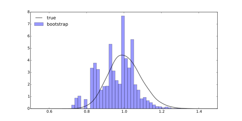
Figure 9.3 shows a histogram of observations from a bootstrap distribution generated using the Julia code above. The underlying sample x1o,…,xNo was created using N=200 IID draws from the LN(0,1) distribution. The statistic used was the sample median. The density shown in the same figure is a numerical approximation of the true sampling distribution of the median over 200 IID draws from the LN(0,1) distribution. The (population) median of the LN(0,1) distribution is 1.
Figure 9.3:Bootstrap draws and sampling distribution for the median
As discussed in Section 9.1.2.1, a good estimator is one that concentrates its probability mass close to the target feature. The extent to which probability mass concentrates is usually measured by the variance or standard deviation of the sampling distribution. The standard deviation is preferable because it comes in units that are easier to interpret.
Because the sampling distribution is typically unknown, so is its standard deviation. Hence we replace the true standard deviation with an estimate. An estimate of the standard deviation of a sampling distribution is usually referred to as the standard error. More generally,
se(γ^):= an estimate of the standard deviation of γ^
This isn’t a proper definition because we haven’t specified which estimate of the standard deviation we are talking about, but nevertheless the terminology is common. One way to compute a standard error of an estimator is to take the sample standard deviation of the bootstrap draws.
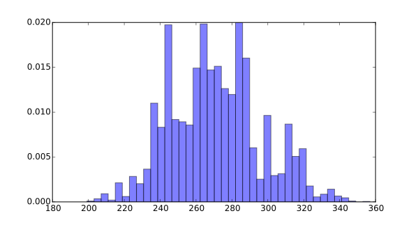
Figure 9.4:Bootstrapped draws for the median of firm sizes by sales
As mentioned above, the standard definition of an estimator does not include any restrictions that imply sensible behavior (as opposed to, say, the definition of a probability). We now turn again to the problem of assessing estimators, following our informal discussion in Section 9.1.2.1. We’ll begin with finite sample properties.
One common criterion for assessing estimators is bias, or lack thereof. Let γ^ be an estimator of a given feature γ=γ(P). The bias of γ^ is defined as
The estimator γ^ is called unbiased for γ over the class of distributions P if
biasP(γ^,γ)=0for all P∈P
The definition is the same when the feature γ and estimator γ^ are vector-valued.
The notation EPγ^ indicates that expectation is taken under the assumption that the data points are IID with common distribution P. In general, the bias depends on P. For example, in the IID setting, the mid-range estimator is unbiased as an estimator of the mean of a uniform distribution on R with unknown end points, but biased for many other distributions, including the lognormal.
Figure 9.2 already suggests bias of the mid-range estimator in the lognormal case. Here’s a simulation in R that provides further confirmation.
> mr <- function(x) return((min(x) + max(x)) / 2)
> observations <- replicate(5000, mr(rlnorm(20)))
> mean(observations)   # Approximate sample mean of mid-range
[1] 3.800108
> exp(1/2)      # Mean of lognormal
[1] 1.648721
Fact 9.2.1 is immediate from linearity of expectations, since
The variance of a given estimator gives a measure of its dispersion. Sensible estimators almost always have the property that the variance goes to zero as N→∞.
Is small variance always desirable for an estimator? If the estimator is biased, then perhaps not, since probability mass might be concentrated in the wrong place. But for an unbiased estimator, low variance is good. It means that probability mass is concentrated around the feature that we wish to estimate.
Low variance is, of course, relative. For example, is the variance in (9.8) low or high? One way to approach this kind of question is to take the class of unbiased estimators of a given feature γ, and find the estimator in the class with the lowest variance. For given γ and given data x1,…,xN, the estimator in the set of unbiased estimators
Uγ:={all statistics γ^ with Eγ^=γ}
that has the lowest variance within this class is called the minimum variance unbiased estimator.
Of course, it’s quite possible that no minimizer exists. Even if it does, it might be hard to determine in practice, or require strong assumptions on the unknown distribution of the data. For these reasons it’s common to focus on smaller classes than Uγ. For example, the estimator in the set of linear unbiased estimators
Uγℓ:={all linear statistics γ^ with Eγ^=γ}
with the lowest variance—if it exists—is called the best linear unbiased estimator.
The theory of minimum variance unbiased estimators and best linear unbiased estimators is traditionally regarded as important. However, there’s no convincing reason to restrict ourselves to unbiased estimators. In fact, as we’ll see, there are good reasons not to.
As for bias, mse(γ^,γ) depends on the joint distribution of the data as well as the specification of γ^, although we haven’t made that dependence explicit in the notation.
Mean squared error is an overall measure of the performance of an estimator that takes into account both bias and variance. In fact in the scalar case we can neatly decompose mean squared error into the sum of variance and squared bias:
This is just (6.3) specialized to the current setting.
As can be seen from both (9.9) and (9.10), when mse(γ^,γ) is small for a given estimator γ^, the estimator concentrates probability mass around the target feature γ. Hence minimizing MSE is a natural and reasonable criterion. In doing so, we are making our subjective loss function explicit, while choosing a loss function that is simple and highly tractable.
When minimizing MSE, we typically find a trade-off between bias and variance: lower variance costs more bias and vice-versa. Moreover solutions usually turn out to be interior. In particular, we can often reduce variance significantly by accepting a small amount of bias.
For most sensible estimators, v converges to zero as the sample size →∞. The message is that unbiased estimators only approach optimality when the data size is large. Here "large" should be understood as relative to model complexity. More complex models need more data to be estimated effectively.
There is a famous example in the theory of statistics due to Stein (1956) that pertains to so-called admissible estimators. Here we’ll borrow Stein’s problem and proposed solution to illustrate several ideas, including the relationship between bias and mean squared error.
To make things concrete, consider the following application: In the field of public finance, one topic of interest is ability-based taxation, which has optimality properties in terms of welfare in certain models. Ability is not observable. Suppose, in particular, that we have a population of K individuals, where the kth individual has idiosyncratic ability μk∈[0,1]. For each agent, we get to observe N noisy signals of ability, each of the form xkn=μk+ϵkn, n=1,…,N. The noise terms ϵkn are all independent N(0,σ2). Our task is to estimate the parameter vector μ=(μ1,…,μK) given the data from the observations xnk. To make things simpler we’ll assume that only μ is unknown.
A natural estimator of μ is the vector sample mean
xˉN=N1∑n=1Nx1n⋮N1∑n=1NxKn
This is the estimator produced by applying the sample analogue principle to our problem. It’s also the maximum likelihood estimator and best linear unbiased.
What Stein showed is that, whenever K>2, there exists an alternative estimator μ^N such that
In other words, μ^N uniformly dominates xˉN in terms of MSE, for all possible values of μ! The estimator in question is what is now known as the James–Stein estimator. It is defined as
μ^N=κxˉNwhereκ:=1−NK−2∥xˉN∥2σ2
This estimator is biased. It achieves lower mean squared error by reducing variance at the expense of a small amount of bias. A relatively simple proof of (9.12) can be found on p. 34 of Young & Smith (2005).
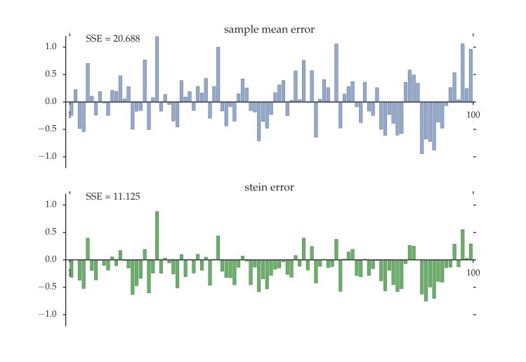
We can get some of the intuition from simulation. In our simulation we set K=200, N=5 and σ=1. Thus we have 5 noisy observations on the ability of each of 200 agents. For each agent we choose their ability μk independently from a uniform distribution on [0,1] and next generate the disturbances ϵkn as independent standard normals. We then compute the estimators xˉN and μ^N and the corresponding error vectors.
Figure 9.5 shows a typical realization. The bars in the top panel are the elements of the vector xˉN−μ, which records the errors for the sample mean estimator xˉN. Those in the lower panel correspond to the errors of the James–Stein estimator. These are noticeably downward biased and also noticeably smaller than the errors of the sample mean estimator. This is reflected in the SSE values in the top left of each panel, which give the sum of squared errors (i.e., the squared norms of the error vectors). The SSE for the sample mean estimator is nearly twice as large.
Let’s now turn to asymptotic properties of estimators. Asymptotic theory concerns whether or not the sampling distribution of a given estimator increasingly concentrates around the feature we wish to estimate, the rate at which this occurs, and the shape of the sampling distribution in large samples.
A fundamental concept in asymptotic statistics is consistency. Let {γ^N} be a sequence of estimators of a given feature γ, based on a sample of size N. We say that γ^N is consistent for γ if
The definition is the same whether the estimators are vector or scalar-valued. The statement that γ^N is consistent means more correctly that the sequence {γ^N} is consistent.
As for bias, whether consistency holds depends not just on γ^N but also on the joint distribution of the data. If we say that γ^N is consistent over a class of distributions P, we mean that (9.13) holds true for any distribution in P.
More generally, γ^N=N1∑n=1Nh(xn) is consistent for γ=∫h(s)P(ds) whenever
x1,…,xN is an IID sample with L(xn)=P for all n and
∫h(s)P(ds) exists.
(See (6.7).) For example, the kth sample moment is consistent for the kth moment over the class of distributions with finite kth moment.
Here’s an example of consistency that requires a bit more work.
Reasonable estimators should be consistent, at least for the IID case. In fact, as we saw in theorem 8.1.1, the entire unknown distribution can be recovered asymptotically with repeated independent samples.
In the IID Gaussian setting of example 9.1.3, the distribution of the sample mean is N(μ,σ2/N). Beyond the information contained in the mean and variance, the fact that the sampling distribution is normal gives us important additional knowledge. We know that the distribution is symmetric, that it has thin tails, and that it puts around 95% of its mass within two standard deviations of the mean. We can determine probabilities of intervals or the expectation of any function of xˉN.
The only concern is our assumption that the observations are Gaussian. Economic theory rarely provides any convincing basis for this assumption. Fortunately, we have the central limit theorem to fall back on, which tells us (remarkably!) that the sample mean is always asymptotically Gaussian, provided that the underlying observations have finite second moment. Even better, the same approximation is valid for many estimators beyond the sample mean.
To clarify, let {γ^N} be a sequence of estimators for some feature γ. We say that γ^N is asymptotically normal if there exists a positive definite matrix Σ such that
When (9.15) holds, Σ is called the asymptotic variance–covariance matrix of γ^N.
Asymptotic normality also implies a rate at which γ^N converges to γ. Indeed, if γ^N is asymptotically normal, then N(γ^N−γ) does not diverge. This means that γ^N−γ goes to zero fast enough to offset the diverging term N. To emphasize this point, we say that an asymptotically normal estimator γ^N is N-consistent for γ.
Still more significant is the fact that asymptotic normality gives us an approximation to the entire sampling distribution. This will provides us with a means of performing inference. Chapter 10 gives details.
We’ve now reviewed the most common methods of assessing estimators. Next we’ll look more deeply at the theory of estimation and decisions under uncertainty. Our focus will be on finite sample properties. This is the most interesting case, since it captures our need to generalize on the basis of limited information.
Despite the efforts of many brilliant statisticians and econometricians, we still lack a convincing general theory of optimality of estimators that rests on purely objective criteria. For example, while the theory of minimum variance unbiased estimators initially seems attractive because it can potentially yield estimators without any subjective judgment on the part of the statistician, there are simple settings where minimum variance unbiased estimators are inadmissible, which means that they fail a minimal requirement for what constitutes a sensible estimator (see below).
Without a fully objective theory of "good" estimators, there are competing notions of what good means, and we are forced to take a stand on what our criteria for assessing estimators are in different situations. This means that the estimation problem is not fully specified until we make our preferences explicit.
For economists it’s natural to think of specifying preference in terms of utility or loss. To fit with modern statistical terminology, we will think in terms of loss. Thus a full description of an estimation problem includes specification of the loss incurred when an estimator performs poorly.
Let’s frame these ideas in line with the seminal work of Wald (1939) and subsequent research on decision theory. A general decision problem consists of
a sample space X,
an action space A,
a set D of decision rules, which are maps d:X→A
a universe Θ of possible states of the world, with typical element θ,
a set of probability distributions {Pθ} over the sample space X, and
a loss function L:A×Θ→R, with interpretation
L(a,θ)=loss incurred by choosing action a when the state of the world is θ.
The state of the world is treated as unknown. The problem is to choose a decision rule d∈D that generates low loss in some sense to be made precise. Central to this discussion is the notion of risk, which is defined as
The integral is over all x∈X. The notation R is used to distinguish this decision-theoretic concept of risk from R(f), the prediction risk of policy f as defined in (8.16).
The problem of choosing estimators is a special case of the decision theory described above. Suppose that we observe data zD taking values in ZD with joint distribution Pθ indexed by θ∈Θ. (The set Θ can be infinite dimensional and θ is just an index.) We wish to estimate some S-valued feature γθ=γ(Pθ) using this data. An estimator in this context is a decision rule γ^ mapping ZD to the action space A=S. If we specify the loss L(γ^,θ) of choosing γ^ when the state of the world is θ, our risk becomes
In the preceding example, the risk of the estimator is its MSE. More generally, if γ^ and γ in (9.20) are vectors and L measures squared vector deviation, then R(γ^,θ)=mse(γ^,γ). Thus, risk gives us a generalization of the idea of evaluating estimators based on MSE, as described in Section 9.2.3. Since loss is subjective, there is no reason we should confine ourselves to quadratic loss.
In the current setup, a natural idea for making optimal decisions—and for choosing optimal estimators, in particular—is to choose decision rules with low risk. The problem with this approach is that the risk depends, in general, on the unknown state of the world θ, and hence the risk-minimizing decision rule also depends on the unknown value θ. In other words, we face Knightian uncertainty. We can’t evaluate risk because we don’t know the probabilities.
This example illustrates the fact that we cannot, in general, choose estimators based on lowest risk in a classical setting. One useful thing we can do, however, is exclude estimators that are always dominated in terms of risk. These are the so-called inadmissible estimators. In particular, a decision rule d is called inadmissible for the general decision problem if there exists a second rule e such that
R(e,θ)⩽R(d,θ) for all θ∈Θ and
R(e,θ)<R(d,θ) for at least one θ∈Θ.
A decision rule that is not inadmissible is called admissible
Another idea that comes out of the desire to minimize risk is minimax. A decision rule dm is called a minimax rule if
r(dm)⩽r(d) for all d∈Dwherer(d):=θ∈ΘsupR(d,θ)
A minimax rule is one that performs well in the worst possible state of the world. Minimax decision rules are an important component of robust control and the study of policy under uncertainty. See, for example, Hansen & Sargent (2008). On the other hand, minimax decision rules can be inadmissible (see, e.g., Young & Smith(2005), p. 9).
The Bayesian approach to statistics leads naturally to a coherent and attractive decision theory. The horse race is not entirely fair, however, since we are granted additional information expressed as a prior. Let’s review the main ideas.
Consider again the generic decision problem discussed above, but now with a prior distribution π=π(θ) over states of the world. In addition each Pθ is now restricted to be a density p(x∣θ). As in Section 8.3.4, we obtain the posterior for θ from the prior given data x via Bayes’ law:
π(θ∣x)=p(x)p(x∣θ)π(θ)(x∈X,θ∈Θ)
Given decision rule d with risk function R(d,θ), the posterior risk or Bayes risk of d is
rπ(d):=∫R(d,θ)π(θ)dθ
A decision rule d that minimizes the Bayes risk is called a Bayes rule. If d is an estimator, then a Bayes rule is called a Bayes estimator. Existence of such rules is not guaranteed, but in many practical instances they are well defined and unique. We give some simple examples below.
There are two particularly attractive features of Bayes rules, and Bayes estimators in particular. One is that Bayes rules are always admissible under mild regularity conditions. See, for example, theorem 10.4.2 of Casella & Berger (2002). A second is that Bayes rules can be computed as a function of observed data, meaning that we don’t have to concern ourselves with how to act in situations that potentially never occur.
To understand the second point, note that we can write the joint density of (x,θ) as either p(x∣θ)π(θ) or π(θ∣x)p(x). Using a change in order of integration followed by this identity, the Bayes risk can be expressed as
This is akin to the scenario encountered in dynamic programming after applying Bellman’s principle of optimality: once we know the value function, we can choose the optimal action just by responding to any observed state.
There are many excellent general texts on statistical inference, including Casella & Berger (2002), Wasserman (2013), and Young & Smith (2005). For a discussion of estimation theory from the perspective of machine learning, see Friedman et al. (2009) or Abu-Mostafa et al. (2012).
DasGupta, A. (2008). Asymptotic Theory of Statistics and Probability. New York: Springer.
Stein, C. (1956). Inadmissibility of the usual estimator for the mean of a multivariate normal distribution. Proceedings of the Third Berkeley Symposium on Mathematical Statistics and Probability, 1(399), 197–206.
Young, G. A., & Smith, R. L. (2005). Essentials of Statistical Inference. Cambridge, UK: Cambridge University Press.
Wald, A. (1939). Contributions to the theory of statistical estimation and testing hypotheses. The Annals of Mathematical Statistics, 10(1), 299–326.
Drenik, A., & Perez, D. J. (2015). Price setting under uncertainty about inflation [Techreport]. New York University.
Hansen, L. P., & Sargent, T. J. (2008). Robustness. Princeton: Princeton University Press.
Casella, G., & Berger, R. L. (2002). Statistical Inference (2nd ed.). Pacific Grove CA: Duxbury.
Wasserman, L. (2013). All of Statistics: A Concise Course in Statistical Inference. New York: Springer.
Friedman, J., Hastie, T., & Tibshirani, R. (2009). The Elements of Statistical Learning (2nd ed.). New York: Springer.
Abu-Mostafa, Y. S., Magdon-Ismail, M., & Lin, H.-T. (2012). Learning from Data. AMLBook.com.