Until now we’ve focused primarily on point estimation. Since data are not infinite, point estimation involves uncertainty. We should not be overconfident in our claim to know the data-generating process. Rather, we should be only as confident as the data allows us to be.
We discussed uncertainty previously when we considered sampling distributions. In this chapter we further quantify estimation uncertainty using the language of confidence sets. We also cover hypothesis tests, which are a second key method of inference in classical statistics.
To tie in with standard presentations we’ll switch to parametric language. The notation is as except that
the marginal distribution of each observation is written as ,
the universe of possible distributions is , and
the joint distribution of the data is written as .
However, we won’t actually restrict ourselves to the case of finitely many parameters. Instead, can be thought of more generally as an index over the set of distributions.
10.1Confidence Sets
Confidence sets are random subsets of model space that contain the true data generating process with high probability. Let’s start with the key definitions and then move on to examples.
10.1.1Finite Sample Confidence Sets
Fix . A random set is called a confidence set for if is observable given the data and, for any ,
Note that it’s the set that’s random here, not .
Confidence sets that are intervals are usually called confidence intervals.
Suppose, for example, that we want to estimate the mean of an unknown distribution based on a set of observations . If we can come up with a 95% confidence set in the sense of (10.1), then we know that the set will contain the mean in about 95% of our experiments, regardless of the underlying distribution.
The last part of the sentence is essential: We don’t know what is, and so the set must be designed such that the probability of containing exceeds regardless of which is generating the data. The difficulty is to actually construct a confidence set with this property for a reasonably large class of distributions. Here’s a traditional approach that uses strong parametric assumptions.
In example 10.1.1, the assumption that is known is clearly unrealistic. If is unknown, a natural approach is to replace this term with the sample standard deviation . In doing so, we will use the following fact, which exercise 10.4.1 asks you to prove.
The random variable (10.3) is called a pivot, which means that its distribution does not depend on the unknown parameters.
Recall that the standard deviation of is . The term is a sample estimate of . Following the discussion in Section 9.1.3.2, we call the standard error of and write it as . We can then write the confidence interval in example 10.1.2 as
10.1.2Asymptotic Methods
While strong parametric assumptions of the form used in examples 10.1.1 and 10.1.2 are difficult to justify in most econometric scenarios, there is another approach to forming confidence intervals that requires much less in terms of structure imposed on the underlying distributions, provided that the sample size is relatively large. Let’s start with a definition: given , a set is called an asymptotic confidence set for if is observable given the data and
for all . Note that is really a sequence of sets and the definition concerns this sequence.
How can we create asymptotic confidence sets? Let’s consider first the case of scalar . Suppose that we have an estimator of that is asymptotically normal for all . Specializing the results in Section 9.2.4.1 to the scalar case, this means that, for all , there exists a positive constant such that
The constant is called the asymptotic variance of . Suppose we have a sequence of statistics such that
As exercise 10.4.2 asks you to show, (10.6) and (10.7) imply that
We can now create our asymptotic confidence intervals as
To see this, take the limit and apply (10.8) to get
10.1.3A Nonparametric Example
Here’s an example of a nonparametric confidence set. In Section 8.1.3 we learned that if is a vector of IID draws from some CDF and is the corresponding ECDF, then converges in probability to . In 1933, A. N. Kolmogorov used an extension of the central limit theorem to obtain an asymptotic distribution for this term. In particular, he showed that when is continuous,
where is the Kolmogorov CDF
As in the CLT, the limiting distribution is independent of the CDF that generates the data.
We can use (10.11) to produce an asymptotic confidence set for . To do so, let be the set of all CDFs on , let be IID draws from , let , and let
The set is an asymptotic confidence set for . Indeed, after rearranging the expression, we get
Applying (10.11) now confirms our claim:
Given our data and the corresponding ECDF , we can present the confidence set visually by highlighting the area between the lower bound and the upper bound over . This is done in figures 10.1 and 10.2. The data are drawn from a -distribution with 10 degrees of freedom and is set to . The values of are 250 for figure 10.1 and 1,000 for figure 10.2.
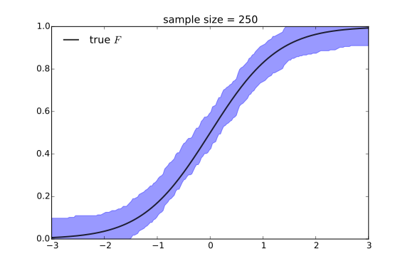
Figure 10.1:Confidence set for the ECDF with 250 observations
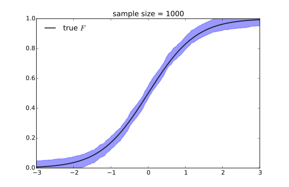
Figure 10.2:Confidence set for the ECDF with 1,000 observations
10.2Hypothesis Tests
This section considers problems of inference where we
hold a belief or theory concerning the probabilities generating the data and
consider whether the data provides evidence for or against that theory.
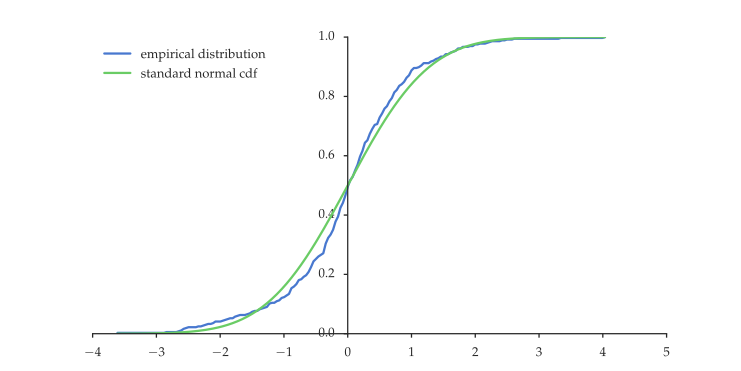
Figure 10.3:ECDF for standardized returns versus the standard normal CDF
To take the next steps, we must formalize the process of setting up a hypothesis and quantifying the extent to which the data points in this or some other direction.
Hypothesis testing begins with the specification of a null hypothesis, which is a statement that the observed data are being generated by a certain model, or one of a certain class of models. One might imagine that the standard procedure in statistics is to show the validity of the null hypothesis but it is not. Rather, a hypothesis test is an attempt to reject the null.
To see why, let’s recall a famous example due to Karl Popper (1902–1994). Consider the claim that all swans are white. It is futile to attempt to prove correctness of this hypothesis: No quantity of white swan sightings can confirm the claim that all swans on planet earth are white. Yet a single black swan can show the claim to be false. In this sense, attempting to falsify a theory on the basis of observation is more constructive than attempting to confirm it.
Although we attempt to reject the null hypothesis, we do so only if strong evidence against it is observed. The rationale is this: Suppose that we have a collection of theories about how the economy works. The procedure would then be to step through the theories, at each stage taking correctness of the theory as the null hypothesis and attempting to reject. If the theory is rejected, then we can discard it. This is a useful process of elimination. However, we don’t want to mistakenly discard a good theory. Hence we only reject when there is strong evidence against the null hypothesis.
10.2.1Constructing Tests
We adopt the setting and notation used in Section 10.1.1. A null hypothesis is a specification of a set of models that we believe the data-generating process belongs to. This amounts to specifying a subset of . The null hypothesis is often written as
If is a singleton, then the null hypothesis is called a simple hypothesis. If not, then the null hypothesis is called a composite hypothesis. A test of the null hypothesis is a test of whether or not the observed data were generated by for some .
Formally, a test of is a binary function mapping the observed data into . The decision rule is
(Failing to reject should not be confused with accepting . More on this below.) Our aim will be to design such that it takes the value when the data present strong evidence against .
The outcome of our test depends on the random sample , and being random, its realization can be misleading. There are two different ways in which the realization can mislead us. First, we can mistakenly reject the null hypothesis when it is in fact true. This is called type I error. Second, we can fail to reject the null hypothesis when it is false. This is called type II error.
The power function associated with the test is the function
Here and below, the symbol indicates that we are computing probabilities under the assumption that . Thus, is the probability that the test rejects when the data are generated by the probabilistic model identified by .
Ideally, we would like when , and when . In practice, this is difficult to achieve.
As discussed above, we tend to be conservative in rejecting the null because we don’t want to discard good theories. For this reason it is traditional to keep the probability of type I error small. Then, if the null is true, our test is unlikely to reject it. Because of this, the standard procedure is to choose a small number such as 0.05 or 0.01, and then adjust the test such that
If (10.14) holds, then the test is said to be of size . Similarly the size of any test with power function is
This is the maximal rejection probability when the null hypothesis is true.
In constructing tests, a common (but not universal) setup is to define a real-valued test statistic and a critical value , and then set
The pair then defines the test, and the rule becomes:
Plots of the power function in (10.17) are presented in figure 10.4 for two different values of . Here is fixed at 10. Since , the size of the test in each case is . Since the power curves are increasing, this is just .
Figure 10.4 illustrates a typical trade-off between type I and type II error. If we increase , we make rejection less likely for all values of . This pushes down type I error, but it also increases the probability that we fail to reject a false null.
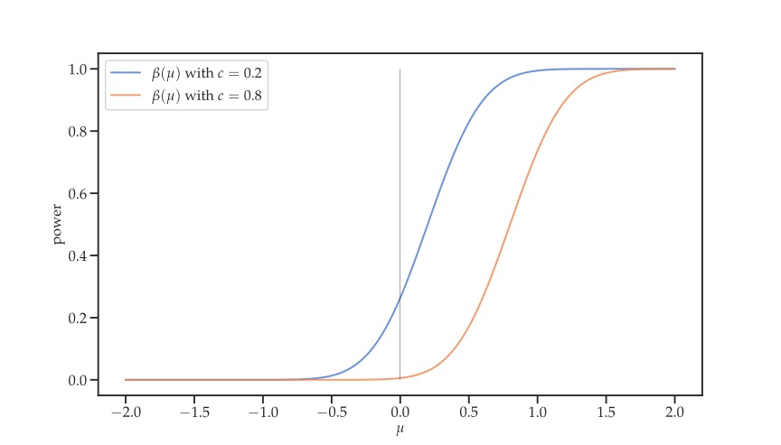
Figure 10.4:Power function
10.2.2Choosing Critical Values
Let’s think a bit more about the test in (10.16). Typically, the choice of is suggested by the problem. For example, if our hypothesis is a statement about the second moment of a random variable, then we might take to be the sample second moment. Once is fixed, we need to adjust such that attains the appropriate size. Thus the standard procedure is to
choose a desired size according to our tolerance for type I error,
identify a suitable test statistic , and
choose a critical value so that is of size .
In performing the last step, we can balance our desire to minimize type II error while maintaining a size test by choosing such that (10.14) holds with equality. In this case, the problem is to choose to solve
Figure 10.5 gives an illustration. In the figure, we’ve taken to be the two element set . The blue line gives an imaginary distribution of , represented as a density, when is generated by . The black line gives the same for . Assuming that a value of is prescribed, our next step is to determine the such that (10.18) holds. Here we choose such that the largest of the two shaded areas is equal to .
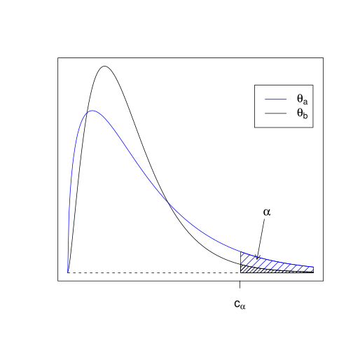
Figure 10.5:Determining the critical value
10.2.3Asymptotic Tests
In general, constructing a test of a given size requires some knowledge of the distribution of the test statistic under the null hypothesis. In many cases, however, we know relatively little about the distribution of the test statistic. Fortunately, we still have options. One approach is to bootstrap. Another is to try to determine the asymptotic distribution of the test statistic. As we’ve learned from the central limit theory, asymptotics hold out the possibility that we can pin down distributions without actually assuming a parametric structure a priori.
To proceed, we need to switch to a notion of asymptotic size for tests, rather than finite sample size. Writing instead of to emphasize the fact that the power function typically depends on sample size, a test is called asymptotically of size if
10.2.3.1A Test for the Empirical Distribution
As another example of how to construct tests which are asymptotically of size , let’s return to the standardized daily returns data presented in figure 10.3. Let be the standard normal CDF as before, and let be that standardized returns are IID draws from . Let be given, and let be the quantile of the Kolmogorov distribution , as defined in (10.12). Finally, let be the ECDF of the data. If the null hypothesis is true, then, by (10.11), we have
For the test
let be the value of the power function when the null hypothesis is true. By (10.22), we have
Hence (10.19) is verified, and the test is asymptotically of size . Notice how the construction of the test inverts the confidence set in Section 10.1.3.
The Nikkei data set used here has 364 observations. The value of the test statistic is 1.548. If , then, as shown in Section 10.1.3, the critical value is 1.36. Hence the test statistic exceeds the critical value, and the null hypothesis is rejected.
While the departure from normality is not easy to see in figure 10.3, it can be seen more clearly in a comparison of the histogram and density, as in figure 10.6. The data are noticeably more peaked and there is evidence of heavy tails.
This application also illustrates how tests often depend on a range of assumptions beyond those that are the focus of a particular hypothesis. Here, for example, a full description of is that standardized returns are IID draws from the standard normal density. The rejection suggests this null is false, but it may be the IID assumption rather than the normality assumption that makes our null a poor fit to the data.[2]
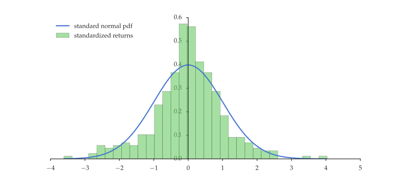
Figure 10.6:Standardized daily returns for the Nikkei 225
10.2.3.2-Values
Typically, a test that rejects at size 0.05 will also reject at size 0.1, but may not reject at size 0.01. Lower means less tolerance for type I error, and forces the critical value to become larger. Hence, for a fixed value of the test statistic, the result of the test may switch from reject to don’t reject. A natural question then is: What is the smallest value of at which we can still reject a given test statistic? This value is called the -value.
To state this more precisely, consider again the setting of Section 10.2. The null hypothesis is and, for each , a test of size . We assume here that is determined via the relationship in (10.18). In this setting, the -value of the test is defined as
Roughly speaking, this is the at which the test switches from reject to don’t reject. Typically, is continuous, and in this case the expression for reduces to
10.2.4Accepting the Null?
Sometimes failure to reject a null hypothesis comes to be seen as presenting evidence in favor of that hypothesis. This is a slippery slope. Here’s one illustration.
In the 1980s econometricians found a new set of toys called unit root tests. First it was discovered that a newly developed test due to Dickey & Fuller (1979) did not reject the null hypothesis of a unit root when applied to a variety of economic time series (Nelson & Plosser (1982)). It was argued that this finding called into question a range of earlier time series methods that assumed trend stationarity, as well as a variety of business cycle studies that assumed stationary innovations around a trend. A raft of new unit root tests appeared. The idea that innovations to major economic time series contain a permanent component became something like a stylized fact.
Let’s think about this carefully. For the sake of concreteness, suppose that we are considering unemployment rate data, where the unit root hypothesis was associated with the concept of hysteresis (see, e.g., Mitchell (1993)). In this setting the unit root null can be expressed most simply as the hypothesis that in the AR(1) process
Here is unemployment, and are parameters and is a zero-mean innovation (see eq. (5) of Mitchell (1993)). Letting be the length of the sample, the standard one-sided Dickey–Fuller test of the unit root null is to
estimate the parameters as and by least squares and
reject the null if , where is a critical value.
Intuitively, when , the test statistic will evaluate to a negative number in large samples. While we omit the derivation, Dickey & Fuller (1979) showed that the test statistic converges in distribution under the null and tabulated critical values for different test sizes.
A number of studies have been unable to reject a unit root null for unemployment rate data (see Mitchell (1993) for an earlier study or Cheng et al. (2012) for a study using a newer set of tests). How should we interpret failure to reject the null in this setting? One possibility is that (10.25) is a good model for the data with . This is not the only possibility, however. Another possibility is that the data are being generated by some other process against which this test has little power.
The second possibility seems more plausible than the first. Indeed, if in (10.25), then as for every bounded -measurable . But employment rates don’t diverge. A more likely story is that while unemployment rates are highly persistent for some range of values, there are equilibrium forces that become increasingly stronger outside this band. For example, the further the unemployment rate falls, the more tightness in the labor market boosts wages, encouraging employers to substitute toward other factors of production and putting upward pressure on the unemployment rate.
We can easily reconcile these equilibrium forces with the idea that the unemployment rate is highly persistent at commonly observed values by adopting a nonlinear model. For example, consider the following simple variation on a random walk:
where is the generalized logistic function depicted in figure 10.7, along with the 45 degree line. For unemployment rates in a band between about 5 and 15, the function has a slope close to one, and the process exhibits strong persistence, just like a random walk. For values above and below this number the shape of causes drift back to the band.
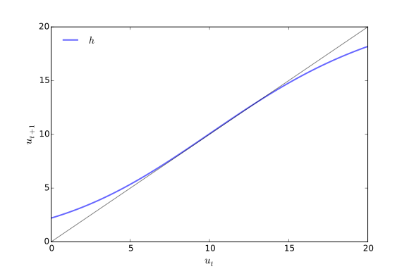
Figure 10.7:A nonlinear process for unemployment dynamics
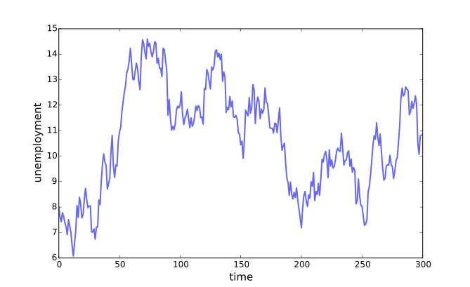
Figure 10.8:Simulated unemployment dynamics
Listing 7 gives code for a simulation when this model generates the data. The shocks are independent Gaussian. In each loop a time series of length 100 is drawn and the Dickey–Fuller test statistic is calculated. The size of the test is set to 0.05, in which case the critical value for the test is (see, e.g., Hayashi (2000), p. 576). If you run the code you will see that for this random seed, the rejection frequency over 5,000 repetitions is around 0.05. This is the same rejection frequency as when the null is true. For this data size, the great majority of tests would fail to reject the unit root model, even though the data-generating process is (10.26).
using LinearAlgebra, Random, Statistics
N, alpha = 100, 0.05  # Length of time series, size of test
critical = -13.7      # Critical value for DF test of size 0.05
Random.seed!(123)     # Set random seed

function h(x, a=0.0, k=22, b=.16, q=0.6, m=10)
    return a + (k - a) / ((1 + q * exp(-b * (x - m)))^(1/q))
end

function dickey_fuller_stat(y)
    y1 = y[1:end-1]
    y2 = y[2:end]
    z2 = y2 .- mean(y2)
    z1 = y1 .- mean(y1)
    rho = dot(z1, z2) / dot(z1, z1)
    return length(y1) * (rho - 1)
end

function sim_dgp(N)
    y = Vector{Float64}(undef, N)
    y[1] = 8  # Initial value of unemployment rate
    for i in 1:N-1
        y[i+1] = h(y[i]) + 0.5 * randn()
    end
    return y
end

M = 5000
rejections = 0
for m in 1:M
    y = sim_dgp(N)
    global rejections += (dickey_fuller_stat(y) < critical)
end
println("Fraction under critical value: ", rejections / M)
Listing 7:DF test applied to a nonlinear time series (Julia)
The interesting thing about this experiment is that the nonlinear data-generating process has very different properties from the null. Not only is it stationary, it is uniformly ergodic, as can be seen by checking the conditions of theorem 16.0.2 of Meyn & Tweedie (2009). This is the strongest possible form of stationarity after the IID property. It means that the effect of initial conditions dies out at a geometric rate that is bounded away from one uniformly over the state space. There is no "permanent component."
10.2.5Statistical Tests in Economics
While the mechanics of hypothesis testing are relatively straightforward, the scientific paradigm based around hypothesis testing is the subject of continual debate. Macroeconomics is an interesting case in point. In the 1970s the rational expectations revolution ushered in a new class of macroeconomic models. One of the first things the proponents of rational expectations did was to test these models against data. Thomas Sargent’s account runs as follows (Evans & Honkapohja (2005)):
My recollection is that Bob Lucas and Ed Prescott were initially very enthusiastic about rational expectations econometrics. After all, it simply involved imposing on ourselves the same high standards we had criticized the Keynesians for failing to live up to. But after about five years of doing likelihood ratio tests on rational expectations models, I recall Bob Lucas and Ed Prescott telling me that those tests were rejecting too many good models.
In the following years, many macroeconomists moved away from formal hypothesis testing. A standard response to classical testing was: “I already know that my model is wrong. Rejection of my model using standard inference tells me nothing new.” For example, Kydland & Prescott (1991) define econometrics as a process without tests:
The main steps in econometric analysis are as follows: defining the question; setting up the model; calibrating the model; and reporting the findings.
How does this line of thinking compare with the standard statistical paradigm? The standard paradigm certainly recognizes that all models are wrong. All sensible models are wrong along some dimensions because they are, by definition, simplified representations of reality. Rejection of models is intended to facilitate survival of the fittest: Those models that explain observed phenomena effectively, and, at the same time, are most difficult to reject, will survive.[3]
At the same time, it’s reasonable to feel sympathy for the frustration with classical hypothesis testing expressed by some economists. While the hypothesis that water boils at 100 degrees C will never be refuted (at least at sea level), in economics even the best models capture only some phenomena of interest. Inevitably they fail to match with reality when viewed in other ways. With enough data almost all sensible economic models can be rejected. But should we discard them? Perhaps some of these models are still useful in guiding our thinking.
How to resolve these different points of view? Some researchers argue that calibration and matching of moments are sufficient as a means of validating their models. But this form of validation imposes little discipline on model builders. Clever economists can find multiple ways to replicate most interesting phenomena observed in the data, each with their own distinct policy implications. More important, the objective of matching moments is largely an in-sample criterion. The dangers of such an approach were illustrated in figure 8.4.
One middle ground is testing of partially specified models, where tests are only concerned with a specific restriction implied by theory. A second path forward is more emphasis on out-of-sample performance in economic studies, which provides a much stricter test of true understanding. A third is offered by the Bayesian approach to model selection, where the emphasis is on comparing and improving models rather than rejection. A fourth is improvements in economic theory, to better match our models to the data.
10.3Further Reading
For a technical discussion of the results surrounding the convergence to the Kolmogorov distribution in (10.12), see section 19.4 of Vaart (2000).
For a discussions of statistical testing in econometrics see, for example, McCloskey & Ziliak (1996) and Freedman (2009). Discussions of calibration in relation to estimation and hypothesis testing can be found in Kydland & Prescott (1991), Kim & Pagan (1999), and many other places. Hansen (2014) presents the main arguments in favor of tests of restrictions in partially specified models. Silver (2012) provides an interesting read on estimation and uncertainty with applications in forecasting.
An excellent summary of unit root tests is given in Hayashi (2000). For a critical overview of unit root testing, see Cochrane (1991).
10.4Exercises
10.4.1Solutions to Selected Exercises
Returns are standardized by subtracting the sample mean and dividing by the sample standard deviation. Data are sourced from the Federal Reserve of St. Louis FRED data set.
The test we’ve implemented can be modified to tackle the case of dependent data. See Negri & Nishiyama (2010) for one such test and more references.
Incidentally, given this description of model selection, it might appear there is an easy way to produce a model that survives forever in the pool of currently acceptable theories, without ever being culled via rejection: just make sure that the model has no testable implications. However, this strategy does not work because a model with no testable implications cannot be considered as a theory of anything. The definition of a scientific theory, as proposed by Karl Popper, is that the theory has one or more testable implications. In other words, the theory can be falsified.
Rhas a built-in function calledchisq.testthat you can use to test your results.In particular, draw each such that for .
- Dickey, D. A., & Fuller, W. A. (1979). Distribution of the estimators for autoregressive time series with a unit root. Journal of the American Statistical Association, 74(366a), 427–431.
- Nelson, C. R., & Plosser, C. R. (1982). Trends and random walks in macroeconmic time series: some evidence and implications. Journal of Monetary Economics, 10(82), 139–162.
- Mitchell, W. F. (1993). Testing for unit roots and persistence in OECD unemployment rates. Applied Economics, 25(12), 1489–1501.
- Cheng, K. M., Durmaz, N., Kim, H., & Stern, M. L. (2012). Hysteresis vs. natural rate of US unemployment. Economic Modelling, 29(2), 428–434.
- Hayashi, F. (2000). Econometrics. Princeton: Princeton University Press.
- Meyn, S. P., & Tweedie, R. L. (2009). Markov Chains and Stochastic Stability (2nd ed.). Cambridge, UK: Cambridge University Press.
- Evans, G. W., & Honkapohja, S. (2005). An interview with Thomas J. Sargent. Macroeconomic Dynamics, 9(4), 561–583.
- Kydland, F. E., & Prescott, E. C. (1991). The econometrics of the general equilibrium approach to business cycles. Scandinavian Journal of Economics, 93(2), 161–178.
- Lucas, R. E. (1978). Asset prices in an exchange economy. Econometrica, 46(6), 1429–1445.
- Van der Vaart, A. W. (2000). Asymptotic Statistics. Cambridge, UK: Cambridge University Press.
- McCloskey, D. N., & Ziliak, S. T. (1996). The standard error of regressions. Journal of Economic Literature, 34(1), 97–114.
- Freedman, D. A. (2009). Statistical Models: Theory and Practice (2nd ed.). Cambridge, UK: Cambridge University Press.
- Kim, K., & Pagan, A. R. (1999). The econometric analysis of calibrated macroeconomic models. In M. H. Pesaran & M. R. Wickens (Eds.), Handbook of Applied Econometrics in Macroeconomics (pp. 356–390). Oxford: Blackwell.
- Hansen, L. P. (2014). Nobel lecture: Uncertainty outside and inside economic models. Journal of Political Economy, 122(5), 945–987.
- Silver, N. (2012). The Signal and the Noise: Why So Many Predictions Fail–But Some Don’t. London: Penguin Press.