11 Regression

11.1Linear Regression¶

Linear regression is one of the core topics of statistics. It is even more central to econometrics, where a shortage of controlled experiments often leaves econometricians trying to factor heterogeneity out ex post. We begin with a nontraditional view of linear regression based on minimal assumptions.

11.1.1The Setup¶

Let’s start with the kind of prediction problem discussed in Section 8.2.2. We study a system with vector input $\boldx_n \in \RR^K$ followed by scalar output $y_n$. For example,

• $\boldx_n$ is a description of a lottery (probabilities, possible outcomes, etc.) in a controlled experiment and $y_n$ is willingness to pay in order to participate (see, e.g., Peysakhovich & Naecker (2015)).

• $\boldx_n$ is a set of household characteristics (ethnicity, age, location, etc.) and $y_n$ is household wealth at some later date (see, e.g., McKernan et al. (2014)).

• $\boldx_n$ is price of electricity, prices of alternatives, temperature, household income, and measurements of the regional income distribution, while $y_n$ is regional electricity consumption (see, e.g., Auffhammer & Wolfram (2014)).

Although we don’t exclude the possibility that $y$ is categorical (i.e., discrete), our loss function will be oriented toward regression (where $y$ takes values in $\RR$).

Suppose that we have $N$ observations $\boldz_n := (\boldx_n,y_n)$, all of which are draws from some fixed joint distribution $P$. Since $P$ is fixed, we are assuming that the system is stationary across the set of draws. Our aim is to predict new output values from input values on the basis of this data. In particular, our problem is to

To define "good predictor" mathematically, we need a loss function. Throughout this chapter we will be using quadratic loss. Thus, in the language of Section 8.2.2, our aim is to minimize the prediction risk

As we saw in Section 5.2.5, the minimizer of (11.2) over the set of all $\bB$-measurable functions is the regression function $f^*(\boldx) := \EEP [y \given \boldx]$. If we could compute this, then all our problems would be solved. But we cannot compute it because $P$ is not known. Instead we apply the principle of empirical risk minimization (see Section 8.2.2), which leads to the problem

Here $\hH$ is the hypothesis space, a set of candidate functions mapping $\RR^K$ into $\RR$. For obvious reasons, the problem (11.3) is called a least squares problem.

If we take $\hH$ to be the set of all functions from $\RR^K$ to $\RR$, then, provided the input vectors are all distinct, we can set the empirical risk $\Remp(f)$ to zero by choosing any function $f$ satisfying $y_n = f(\boldx_n)$ for all $n$. However, as discussed at length in Section 8.2.3, minimizing empirical risk is different from minimizing the prediction risk $R(f)$. The latter is what we actually want to minimize. Thus $\hH$ must be restricted.

In this chapter we consider the case $\hH = \llL$, where $\llL$ is all linear functions from $\RR^K$ to $\RR$. Recalling theorem 3.1.1, we can write

The problem (11.3) then reduces to

The term $\frac{1}{N}$ has been dropped because it does not affect the minimizer. This is the multivariate version of (8.22).

The idea of choosing $\boldb$ to minimize (11.5) is intuitive: We are choosing a "line of best fit" to minimize in-sample prediction error. This optimization problem has a long tradition. It dates back at least as far as Carl Gauss’s work on the orbital position of Ceres, published in 1801.

You might be wondering whether the choice $\hH = \llL$ is a suitable one. This is an excellent question. It might not be. However, there are good reasons to start with $\llL$, even in this setting where no linearity assumptions are imposed. First, $\llL$ is a natural starting point when seeking a class of simple, well-behaved functions. Second, as we’ll see, setting $\hH = \llL$ allows us to obtain an analytical expression for the minimizer, which simplifies both analysis and computation. Third, the technique has an extension from $\llL$ to broader classes of functions, as described in Section 11.2.1.

11.1.2The Least Squares Estimator¶

Now let’s solve (11.5). With our knowledge of overdetermined systems (see Section 3.3.2), we already have all the necessary tools. This will be more obvious after we switch to matrix notation. To do this, let

and

Sometimes $\boldX$ is called the design matrix. By construction, $\col_k \boldX =$ all observations on the $k$th regressor. Also, for any $\boldb \in \RR^K$, we have

It follows that the objective function in (11.5) can be written as

Since strictly increasing transforms preserve the set of minimizers (see Section 15.4),

We already know how to solve for the minimizer on the right-hand side of (11.8). By theorem 3.3.2, the solution is

Traditionally, this random vector $\hboldbeta$ is called the least squares estimator. Once we move to more classical assumptions it will be an estimator of a particular parameter vector. At this stage it just defines our answer to the problem posed in (11.1). That is,

In terms of geometric interpretation, since $\boldX \hboldbeta$ solves (11.8), it is the closest point in $\colspace \boldX$ to $\boldy$. In particular,

(See (3.13).) In what follows, $\boldM$ is the residual projection, as defined in (2.11).

11.1.2.1Assumptions¶

Theorem 3.3.2 and our definition of $\hboldbeta$ in (11.9) require that $\boldX$ has full column rank (or, equivalently, that the columns of $\boldX$ are linearly independent—see page ).

By theorem 2.1.3, $N \geq K$ is a necessary condition for assumption 11.1.1 to hold. (If $N < K$, then $\RR^N$, which is necessarily spanned by $N$ vectors, cannot contain $K$ linearly independent vectors.)

If assumption 11.1.1 fails, then a minimizer of (11.8) still exists but is no longer unique (see ex. 3.5.34). While we can treat this case, it rarely occurs in well-designed regression problems.

Let’s also put some mild regularity conditions on the common joint distribution $P$ of each data point $\boldz_n := (\boldx_n, y_n)$.

Finite second moments are imposed because we want to evaluate expected squared errors. This assumption cannot be weakened unless we are willing to work with a different loss function. Positive definiteness of $\Sigmax$ ensures that the asymptotic limit of our estimator is well defined.^[1]

11.1.2.2Notation¶

There’s a range of standard notation associated with linear least squares estimation. Let’s collect it in one place. First, the projection

is called the vector of fitted values. The $n$th fitted value $\hat y_n$ is the prediction $\boldx_n^\T \, \hboldbeta$ associated with least squares estimate and the $n$th observation $\boldx_n$ of the input vector. The vector $\boldM \boldy$ is often denoted $\hboldu$, and called the vector of residuals:

The vector of residuals corresponds to the error that occurs when $\boldy$ is approximated by $\boldP \boldy$. From fact 2.2.8 we have

In other words, $\boldy$ can be decomposed into two orthogonal vectors $\boldP \boldy$ and $\boldM \boldy$, where the first represents the best approximation to $\boldy$ in $\colspace \boldX$, and the second represents the residual.

Related to the fitted values and residuals, we have some standard definitions:

• Total sum of squares $:= \tss := \| \boldy \|^2$.

• Residual sum of squares $:= \rss := \| \boldM \boldy \|^2$.

• Explained sum of squares $:= \ess := \| \boldP \boldy \|^2$.

By (11.11) and the Pythagorean law,

When running regressions it is conventional to report the coefficient of determination, or $R^2$. The plain vanilla definition of $R^2$ is

Many regression packages report an alternative definition of $R^2$. See Section 11.2.3 below.

11.1.3Out-of-Sample Fit¶

We have stressed a number of times that learning from data (statistics) means generalization from current observations to new ones. As such, the most important measure of success for a statistical procedure is out-of-sample fit. So how does linear least squares perform out-of-sample? We start with a general observation about linear predictors.

Here $f^*$ is the regression function and $\boldb^* = \Sigmax^{-1} \, \EE[\boldx \, y]$ is the vector of coefficients in the best linear predictor . $R(f)$ is the prediction risk of $f$ and expectations are taken under the unknown joint distribution $P$ of the pairs $(\boldx, y)$.

The proof of theorem 11.1.1 is given in Section 11.1.3.1. For now let’s look at interpretation. The general question is how well we can generalize (i.e., reduce prediction risk) using linear functions. Theorem 11.1.1 decomposes the prediction risk of an arbitrary linear predictor $\ell (\boldx) = \boldx^\T \boldb$ into three terms:

The intrinsic risk is also called Bayes risk (see example 8.2.3). It is the residual error after $y$ is approximated with the best possible predictor (i.e., the regression function). It is large to the extent that $y$ is hard to predict using $\boldx$.

The approximation error or bias is the deviation between the best predictor and the best linear predictor. It reflects the cost of our decision to approximate the regression function using a linear architecture. If this architecture is held fixed, the approximation error is also fixed and cannot be reduced in the estimation process.

The estimation error is caused by the deviation of our estimator from the best linear predictor $\boldb^*$. This deviation occurs because we are predicting using finite sample information on the joint distribution of $(\boldx, y)$.

Theorem 11.1.1 tells us that once $\hH$ is set to the class of linear functions, the best we can do is find an estimation method (a learning algorithm) that produces an estimate that is close to $\boldb^*$ on average when the sample size is sufficiently large. The next result states that the least squares estimator $\hboldbeta$ has this property.

The proof is below. Independence is required only for the LLN to function. We could weaken this to ergodicity (see Section 7.1.1) and obtain the same conclusion.^[2]

On one level, theorems 11.1.1 and 11.1.2 are reassuring. They tell us that if the underlying process is relatively linear, then we will attain small risk asymptotically. On the other hand, the Glivenko–Cantelli theorem tells us that we can learn everything about the underlying distribution in the limit. Here we are bounded away from this kind of consistency whenever the approximation error is positive.

As will be discussed in chapter 14, a general principle of induction is that we should introduce bias in finite samples to avoid overfitting, while at the same time reducing bias asymptotically, as the empirical distribution converges to the true distribution. By comparison, in standard linear regression the bias is held fixed by the linearity assumption.

11.1.3.1Proofs¶

11.1.4In-Sample Fit¶

In-sample fit measures how well a given model fits the same data set that it was estimated on. The difference between in-sample fit (empirical risk) and out-of-sample fit (risk) was discussed in Section 8.2.3. In-sample fit of a regression is often measured with $R^2$ (see (11.13)). Let’s make some further comments on $R^2$ and then discuss how $R^2$ relates to in-sample fit.

That $R^2 \leq 1$ is immediate from $\| \boldP \boldy \| \leq \| \boldy \|$ (cf. theorem 2.2.2). Exercise 11.4.17 asks you to prove the second claim. More generally, a high $R^2$ indicates $\boldy$ is relatively close to $\colspace \boldX$. This fact suggests that we can increase $R^2$ at least weakly by adding regressors. As we do so the column space of $\boldX$ expands, pushing out towards $\boldy$. Here’s a formal statement:

For a proof, see exercise 11.4.8 and its solution.

High $R^2$ is sometimes equated with successful regression. This is a misunderstanding of the aim of statistics. The correct definition of statistical learning is effective generalization from existing data. In the present context this means that the linear predictor produced by regression attains low risk.

So how does $R^2$ relate to risk? What $R^2$ actually measures is the degree to which empirical risk is minimized. To see this, note that

where $\Remp$ is as defined in (11.3) and $\hat f$ is our linear predictor $\hat f(\boldx) = \boldx^\T \hboldbeta$. Thus high $R^2$ means low empirical risk and good in-sample fit. But low empirical risk is no guarantee of low prediction risk, as was emphasized in Section 8.2.3.

Here’s a simulation that shows how we can produce high $R^2$ without estimating anything meaningful. We take $x_n$ and $y_n$ as independent draws from a uniform distribution on $[0,1]$. By construction, there is no relationship between these two variables. For the regressors we take the powers $1, x, x^2, \ldots, x^K$, where $K$ is a positive integer. The R code below runs these regressions for different values of $K$. At $K=25$ the value of $R^2$ is around 0.95. This is despite the fact that no relationship exists between $x$ and $y$.

set.seed(1234)
N <- 25
y <- runif(N)
x <- runif(N)
X <- rep(1, N)

Kmax <- 25
for (K in 1:Kmax) {
    X <- cbind(X, x^K)
    results <- lm(y ~ 0 + X)
    Py2 <- sum(results$fitted.values^2)
    y2 <- sum(y^2)
    cat("K =", K, "R^2 =", Py2 / y2, "\n")
}

To finish this section, let’s draw a connection between fact 11.1.2, which says that the value of $R^2$ is at least weakly increasing in the number of right-hand side variables, and fact 8.2.1. Suppose that $\boldx$ lists a large number of possible regressors. Let the hypothesis space be

Here $1 \leq j \leq K$. Empirical risk minimization over $\hH_j$ is equivalent to linear regression over the first $j$ regressors. Empirical risk falls as $j$ increases by fact 8.2.1. Hence $R^2$ increases. This is the same conclusion as fact 11.1.2.

11.2The Geometry of Least Squares¶

In this section we cover transformations of the data and an important theorem on subsets of the least squares estimator.

11.2.1Transformations and Basis Functions¶

In discussing the decision to set $\hH = \llL$ in Section 11.1.1, we mentioned that we can use many of the same ideas when extending $\hH$ to a broader class of functions. The idea is to first transform the data using some arbitrary function $\boldphi \colon \RR^K \to \RR^J$. The action of $\boldphi$ on $\boldx \in \RR^K$ is

The individual functions $\phi_1, \ldots, \phi_J$ mapping $\RR^K$ into $\RR$ are sometimes called basis functions. In machine learning texts, the range of $\boldphi$ is called feature space. Linear least squares is now applied in feature space. That is, we solve the empirical risk minimization problem when the hypothesis space is

The empirical risk minimization problem is then

Switching to matrix notation, if

then the objective in (11.19) can be expressed as $\| \boldy - \boldPhi \boldgamma \|^2$. Since increasing functions don’t affect minimizers, the problem becomes

Assuming that $\boldPhi$ is full column rank, the solution is

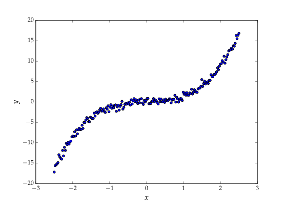
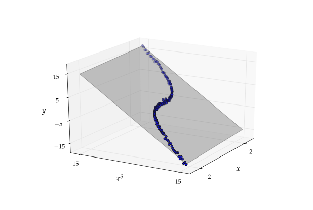
Figure 11.1 and Figure 11.2 help illustrate how transformations can reduce approximation error. In figure 11.1 it is clear that no linear function mapping $x$ to $y$ can produce small approximation error. Figure 11.2 shows the data after applying the transformation $\RR \ni x \mapsto \boldphi(x) := (x, x^3)^\T \in \RR^2$. The plane drawn in figure 11.2 represents a linear function $\ell \colon \RR^2 \to \RR$. The composition $\ell \circ \boldphi$ has low approximation error. The two figures illustrate how nonlinear data can become linear when projected into higher dimensions.

Below, when $y$ is regressed on $\boldx$, we can imagine that the data have already been transformed, and $\boldx$ is the result. Hence we use $\boldX$ to denote the design matrix instead of $\Phi$ without loss of generality.

11.2.2The Frisch–Waugh–Lovell Theorem¶

The Frisch–Waugh–Lovell (FWL) theorem yields an expression for an arbitrary sub-vector of the least squares estimator $\hboldbeta$ obtained by regressing $\boldy$ on $\boldX$. In stating the theorem, we continue with the assumptions of Section 11.1. Let $\boldy$ and $\boldX$ be given and let $\hboldbeta$ be as in (11.9). In addition, let $K_1$ be an integer with $1 \leq K_1 < K$, and let

• $\boldX_1$ be a matrix consisting of the first $K_1$ columns of $\boldX$,

• $\boldX_2$ be a matrix consisting of the remaining $K_2 := K - K_1$ columns,

• $\hboldbeta_1$ be the $K_1 \times 1$ vector consisting of the first $K_1$ elements of $\hboldbeta$.

• $\hboldbeta_2$ be the $K_2 \times 1$ vector consisting of the remaining $K_2$ elements of $\hboldbeta$,

• $\boldP_1 := \proj ( \colspace \boldX_1)$, and

• $\boldM_1 := \boldI - \boldP_1 =$ the corresponding residual projection.

As exercise 11.4.22 asks you to show, the expression for $\hboldbeta_2$ in theorem 11.2.1 can be rewritten as

Close inspection of this formula confirms the following claim: There is another way to obtain $\hboldbeta_2$ besides just regressing $\boldy$ on $\boldX$ and then extracting the last $K_2$ elements: we can also regress $\boldM_1 \boldy$ on $\boldM_1 \boldX_2$ to produce the same result.

To get some feeling for what this means, let’s look at a special case, where $\boldX_2$ is the single column $\col_K \boldX$, containing the observations on the $K$th regressor. To tie into this notation let’s write $\boldX_1$ as $\boldX_{-K}$ to remind us that it stands for all columns of $\boldX$ expect the $K$th one, and similarly for $\boldM_1$. In view of the preceding discussion, the least squares estimate $\hat \beta_K$ can be found by regressing

on

Loosely speaking, these two residual terms $\tilde \boldy$ and $\tilde \boldx_K$ can be thought of as the parts of $\boldy$ and $\col_K \boldX$ that are “not explained by” $\boldX_{-K}$. Thus, on an intuitive level, the process for obtaining the least squares estimate $\hat \beta_K$ is as follows:

This is obviously different from the process for obtaining the coefficient of the vector $\col_K \boldX$ in a simple univariate regression, the latter being just

In words, the difference between the univariate least squares estimated coefficient of the $K$th regressor and the multiple regression least squares coefficient is that the multiple regression coefficient $\hat \beta_K$ measures the isolated relationship between $x_K$ and $y$, without taking into account indirect channels involving other variables.

We can illustrate this idea further with a small simulation. Suppose that

If we generate $N$ independent observations from this model and regress $y$ on the observations of $(x_1, x_2)$, then, provided that $N$ is sufficiently large, the coefficients for $x_1$ and $x_2$ will both be close to unity (see theorem 11.1.2). However, if we regress $y$ on $x_1$ alone, then the coefficient for $x_1$ will depend on the relationship between $x_1$ and $x_2$. For example:

> N <- 1000
> x1 <- runif(N)
> x2 = 10 * exp(x1) + rnorm(N)
> y <- x1 + x2 + rnorm(N)
> results <- lm(y ~ 0 + x1)
> results$coefficients
      x1 
      30.83076 

Here the coefficient for $x_1$ is much larger than unity, because an increase in $x_1$ tends to have a large positive effect on $x_2$, which in turn increases $y$. The coefficient in the univariate regression reflects this total effect.

11.2.2.1Application: Simple Regression¶

Here’s an easy application of the FWL theorem: deriving the familiar expression for the slope coefficient in simple linear regression (see Section 8.2.1.1) from the multivariate expression. Simple linear regression is a special case of multivariate regression when $\boldone$ is the first column of $\boldX$ and $K = 2$. In this section, the second column of $\boldX$ will be denoted by $\boldx$. As we saw in (8.14), the least squares estimates are

where $\bar x$ is the sample mean of $\boldx$ and $\bar y$ is the sample mean of $\boldy$. We can rewrite the slope coefficient $\hat \beta_2$ more succinctly as

By the FWL theorem (equation (11.25)), we also have

where $\boldM_c$ is the residual projection associated with the linear subspace $S = \Span\{\boldone\}$, as defined in (3.10). For this residual projection $\boldM_c$ and any $\boldz$, we have $\boldM_c \boldz = \boldz - \bar z \boldone$. Hence the right-hand sides of (11.28) and (11.29) coincide.

11.2.3Centered Observations¶

Let’s generalize the preceding discussion to the case where there are multiple nonconstant regressors. The only difference is that instead of one column $\boldx$ of observations on a single nonconstant regressor, we have a matrix $\boldX_2$ containing multiple columns, each a vector of observations on a nonconstant regressor. If the least squares estimate $\hboldbeta$ is partitioned into $(\hat \beta_1, \hboldbeta_2)$, then we can write

Applying the FWL theorem (equation (11.25)) once more, we can write $\hboldbeta_2$ as

where $\boldM_c$ is the residual projection in (3.10). As we saw in the last section, $\boldM_c \boldy$ is $\boldy$ centered around its mean. Similarly, $\boldM_c\boldX_2$ is a matrix formed by taking each column of $\boldX_2$ and centering it around its mean. It follows that in a least squares regression with an intercept, the estimated coefficients of the nonconstant regressors are equal to the estimated coefficients of a zero-intercept regression performed after all variables have been centered around their mean.

Let’s use some related ideas to discuss an alternative to the coefficient of determination introduced in (11.13). There are several versions of $R^2$ reported in common regression packages. One of these is so called centered $R^2$. The version in (11.13) will henceforth be called the uncentered $R^2$ for clarity.

One motivation for introducing an alternative to uncentered $R^2$ is that it fails to be invariant to certain changes of units. While it is invariant to changes of units that involve rescaling of the regressand $\boldy$ (see ex. 11.4.2), it is not invariant to changes of units that involve addition or subtraction (actual inflation versus inflation in excess of a certain level, income versus income over a certain threshold, etc.) whenever $\boldX$ contains an intercept. Exercise 11.4.3 asks you to prove this.

This is one reason many econometricians use the centered $R^2$ rather than $R^2$, at least when the regression contains an intercept. For the purposes of this section, let’s assume that this is the case (or, more generally, that $\boldone \in \colspace \boldX$). Centered $R^2$ is defined as

$\boldM_c$ is as defined in (3.10). The equality of the two expressions for $R^2_c$ is left as an exercise (ex. 11.4.6). Adding a constant to each element of $\boldy$ will have no effect on $R^2_c$ because $\boldM_c$ maps constant vectors to $\boldzero$ (see example 3.3.1).

Centered $R^2$ can be rewritten (ex. 11.4.7) as

It is a further exercise (ex. 11.4.5) to show that, in the case of the simple regression, the $R_c^2$ is equal to the square of the sample correlation between the regressor and regressand, as defined in (8.5). Thus $R_c^2$ is a measure of correlation.

11.3Further Reading¶

For additional references on the material covered in this chapter see, for example, Friedman et al. (2009), Ruud (2000), Cameron & Trivedi (2005), or Davidson & MacKinnon (2004).

11.4Exercises¶

11.4.1Solutions to Selected Exercises¶