12 Ordinary Least Squares

In chapter 11 we imposed only mild regularity conditions on the data. To further investigate linear least squares estimation and provide additional interpretation of the estimated coefficients, we need to make more assumptions. The purpose of this chapter is to describe the properties of linear least squares estimation under the classical OLS assumptions, where OLS stands for ordinary least squares.

12.1Estimation under OLS¶

In this section we introduce the OLS assumptions and study the finite sample properties of the OLS estimators under these assumptions.

12.1.1Assumptions¶

Let $\boldX$ and $\boldy$ be as defined in Section 11.1. The OLS assumptions are as follows:

Let’s break these assumptions down and see what they imply.

Assumption 12.1.1 is just a repetition of assumption 11.1.1 from chapter 11. Assumption 12.1.2 can be decomposed into the separate equations

Here are some examples of models that produce relationships in the form of (12.1).

The notation in fact 12.1.1 follows Section 11.1.2.2. Exercise 12.4.2 requests a proof.

Exercise 12.4.3 asks you to give proofs.

Parts (ii) and (iii) are called homoskedasticity and zero correlation respectively.

Combining assumptions 12.1.3 and 12.1.4 gives

Thus the conditional variance–covariance matrix is the diagonal matrix $\sigma^2 \boldI$.

12.1.2The OLS Estimators¶

The standard estimator of $\boldbeta$ in (12.1) is the least squares estimator $\hboldbeta$ defined in (11.9). That is,

Unlike chapter 11, it’s now understood as an estimator of the unknown parameter vector $\boldbeta$. In this context, $\hboldbeta$ is also called the OLS estimator of $\boldbeta$. Substituting $\boldy = \boldX \boldbeta + \boldu$ into (12.3) and cancelling terms gives the useful comparison

The usual OLS estimator of the parameter $\sigma^2$ introduced in assumption 12.1.4 is

While we can compute $\hboldbeta$ and $\hat \sigma^2$ directly using the expressions in (12.3) and (12.5), in practice it’s more common to pass them to a routine in a regression package. Here’s an example that runs the gravity model regression (12.2) on world trade data using Python.

First we import some Python libraries often used for statistics:

from numpy import log  # used in the formula below
import pandas as pd, statsmodels.formula.api as smf

Then we read in the data to a pandas DataFrame from a local CSV file:

data = pd.read_csv("./data/gravity_dataset_2013.csv")

Next we build a model using a formula to indicate the regression we want to run symbolically (similar to R).

formula = "log(value) ~ log(egdp) + log(igdp) + log(dist)"
model = smf.ols(formula, data)

The formula used above is analogous to (12.2). We omit the shock (the last term in (12.2)) because it is not part of the data set, as well as the constant term, which is included automatically. The names egdp and igdp represent exporter and importer GDP respectively.

Now we can perform the estimation and print a table summarizing results:

result = model.fit(cov_type='HC1')
print(result.summary())

The output is as follows:

                            OLS Regression Results                            
==============================================================================
Dep. Variable:             log(value)   R-squared:                       0.652
Model:                            OLS   Adj. R-squared:                  0.652
Method:                 Least Squares   F-statistic:                 1.203e+04
Date:                Wed, 04 Nov 2015   Prob (F-statistic):               0.00
Time:                        16:02:42   Log-Likelihood:                -47185.
No. Observations:               19655   AIC:                         9.438e+04
Df Residuals:                   19651   BIC:                         9.441e+04
Df Model:                           3                                         
Covariance Type:                  HC1                                         
==============================================================================
                 coef    std err          z      P>|z|      [95.0% Conf. Int.]
------------------------------------------------------------------------------
Intercept    -30.2350      0.394    -76.773      0.000       -31.007   -29.463
log(egdp)      1.2783      0.008    153.772      0.000         1.262     1.295
log(igdp)      1.0287      0.009    118.885      0.000         1.012     1.046
log(dist)     -1.3483      0.023    -58.113      0.000        -1.394    -1.303
==============================================================================
Omnibus:                     1819.031   Durbin-Watson:                   1.798
Prob(Omnibus):                  0.000   Jarque-Bera (JB):             3361.159
Skew:                          -0.639   Prob(JB):                         0.00
Kurtosis:                       4.571   Cond. No.                         708.
==============================================================================

The value of the OLS estimate $\hboldbeta$ is the column under coef. Objects such as standard errors are discussed below. The argument cov_type=’HC1’ to the model.fit call that produced this table requests heteroskedasticity-consistent or "robust" standard errors, which will be discussed in Section 12.2.1.

Let’s check that the values for $\hboldbeta$ reported under coef coincide with the expression for $\hboldbeta$ given in (12.3). First we build the design matrix $\boldX$ (see the URL given above for details) and then compute as follows:

betahat = inv(X.T @ X) @ X.T @ y

When we print the result the output agrees with the output in the table

[-30.23498073   1.27825004   1.02865139  -1.34830012]    

The expression for the $R^2$ in the table above is for $R_c^2$, as given in (11.31).

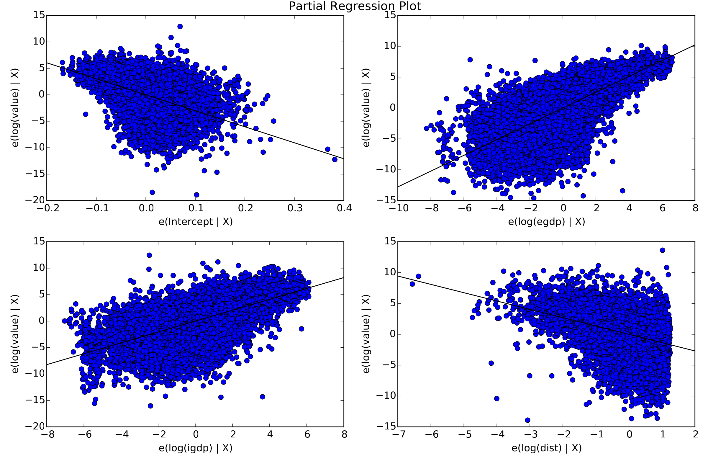
Figure 12.1 shows a partial regression plot for the linear model just described. It is produced from the result object generated above via the commands

import matplotlib.pyplot as plt
import statsmodels.api as sm
fig = plt.figure()
fig = sm.graphics.plot_partregress_grid(result, fig=fig)

To understand the figure, consider, for example, the bottom left subplot, which shows the relationship between log(igdp) and the dependent variable. The data points in the plot correspond to the residuals in (11.26) and (11.27). In particular, the values on the horizontal axis are the residuals from regressing log(igdp) on all other columns in $\boldX$, while those on the vertical axis are the residuals from regressing the dependent variable log(value) on all other columns in $\boldX$.

The relationship between these residuals measures the change in log(value) associated with changing log(igdp) while holding all other variables fixed. The slope of the regression line running through the plot is exactly the coefficient estimate on log(igdp). For clarification see the discussion surrounding (11.26) and (11.27).

The partial regression plot can be useful both for interpretation and diagnostics. For now, however, let’s look at some general theory concerning properties of the OLS estimators.

12.1.3Finite Sample Properties¶

Let’s start with classical results on finite sample properties under the OLS assumptions. These are elegant results, although you should also read Section 14.2 if you want to view them with proper perspective. Our first result shows that, under the OLS assumptions, the OLS estimators are unbiased.

Now that we know $\hboldbeta$ is unbiased, let’s consider the variance.

For a proof, see exercise 12.4.5 and its solution.

Is the value on the right-hand side of (12.8) small or large? A famous result in OLS theory is that under the stated conditions, the OLS estimator $\hboldbeta$ is best linear unbiased. That is, in the class of linear unbiased estimators of $\boldbeta$, the OLS estimator has the lowest variance.

Here $\var [\hboldbeta \given \boldX] \leq \var [\boldb \given \boldX]$ means that $\var [\boldb \given \boldX] - \var [\hboldbeta \given \boldX]$ is nonnegative definite. Since matrices have no standard ordering, this is one way to assert that $\var [\boldb \given \boldX]$ is “larger.” One implication is that $\var [b_k \given \boldX] \geq \var [\hat \beta_k \given \boldX]$ for all $k$. (Why?)

Also, linearity of $\boldb$ means that $\boldb$ is linear as a function of $\boldy$, taking $\boldX$ as fixed. In view of theorem 3.1.1, this is equivalent to requiring that $\boldb = \boldC \boldy$ for some matrix $\boldC$. The matrix $\boldC$ is allowed to depend on $\boldX$ but not $\boldy$.

The statement that $\boldb$ is unbiased means $\EE [\boldb \given \boldX] = \EE [ \boldC \boldy \given \boldX] = \boldbeta$ for all $\boldbeta \in \RR^K$.

12.1.3.1Precision of the Estimates¶

Theorem 12.1.2 shows that the variance–covariance matrix of $\hboldbeta$ given $\boldX$ is $\sigma^2 (\boldX^\T \boldX)^{-1}$. The scalar variances of the individual OLS coefficient estimates $\hat \beta_1, \ldots, \hat \beta_K$ are given by the principal diagonal of this matrix. Since each $\hat \beta_k$ is unbiased (theorem 12.1.1), small variance means probability mass concentrated around the true parameter $\beta_k$. In this case, we say that the estimator has high precision.

The Gauss–Markov theorem states that, as far as unbiased linear estimators go, the OLS estimates will have highest precision. But what if we hold the estimation technique fixed, as well as the sample size, and vary the application? Which problems will have high precision estimates, and which will have low precision estimates?

To answer this question, let’s focus on the variance of a fixed coefficient $\beta_k$. We can write $\boldy = \boldX \boldbeta + \boldu$ as

where $\col_k(\boldX)$ is the vector of observations of the $k$th regressor, $\boldX_1$ contains as its columns the observations of the other regressors, and $\hboldbeta_1$ is the OLS estimates of the corresponding coefficients. By the FWL theorem,

where $\boldM_1$ is the residual projection $\boldM_1 := \boldI - \boldP_1$ and $\boldP_1 := \boldX_1 (\boldX_1^\T\boldX_1)^{-1} \boldX_1^\T$ projects onto $\colspace \boldX_1$. Applying $\boldM_1$ to both sides of (12.10) yields

Substituting into (12.11) gives

Some calculations then show (ex. 12.4.11) that

Thus the variance of $\hat \beta_k$ depends on two components, the variance $\sigma^2$ of the shock $u$ and the norm of the vector $\boldM_1 \col_k \boldX$.

The variance in $\sigma^2$ is unavoidable: some data are noisier than others. The larger the variance in the unobservable shock, the harder it will be to estimate $\beta_k$ with good precession.

The other term is more interesting. $\boldM_1 \col_k \boldX$ is the residuals from regressing $\col_k \boldX$ on $\boldX_1$, and $\|\boldM_1 \col_k \boldX\|$ is the norm of this vector. If this norm is small, then the variance of $\hat \beta_k$ will be large.

When will this norm be small? It will be so when $\col_k \boldX$ is “almost” a linear combination of the other regressors and hence close to $\colspace \boldX_1$. Then

This situation is sometimes referred to as multicollinearity.

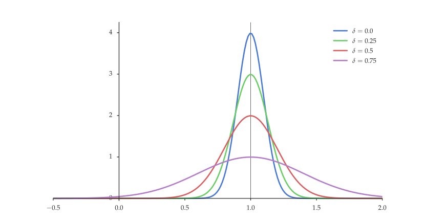
Figure 12.2 gives an illustration of the effect of multicollinearity on the variance of OLS estimate $\hat \beta_2$. In this example $\boldX$ has two columns. They are related by $\col_2 \boldX = \delta \col_1 \boldX + (1 - \delta) \boldz$, where $\boldz$ is a vector of $N$ independent draws from the standard normal distribution. Larger $\delta$ means more dependence between $\col_1 \boldX$ and $\col_2 \boldX$. The true parameter is $\beta_2 = 1$. The figure shows the distribution of $\hat \beta_2$ for different values of $\delta$. The estimator $\hat \beta_2$ is unbiased but its variance increases with $\delta$. (The normal shape of the distribution is explained in the next section.)

12.1.4Inference with Normal Errors¶

If we want to compute confidence intervals or test hypotheses about the coefficients in finite samples (i.e., without appealing to asymptotics), we need to strengthen our OLS assumptions even further, by specifying the parametric class of the error vector $\boldu$. Because of its many attractive properties, the normal distribution is the default.

Assumption 12.1.5 implies both assumption 12.1.3 and assumption 12.1.4. It also implies that the conditional distribution of $\hboldbeta$ given $\boldX$ is normal, as can be seen from (12.4) and fact 5.1.5. The next theorem records this result.

It follows from theorem 12.1.4 and (5.12) that the distribution of individual coefficient $\hat \beta_k$ given $\boldX$ is also normal, with

Here $v_k (\boldX) :=$ the $(k,k)$th element of $(\boldX^\T \boldX)^{-1}$.

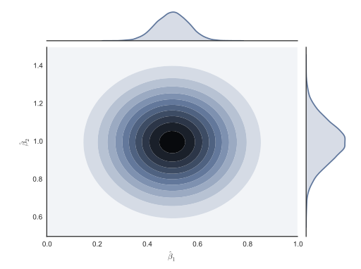
Theorem 12.1.4 and the normality of the marginal distributions along the individual coefficients is illustrated in figure 12.3. The central plot shows the contours of a density estimate that can be understood as a smoothed histogram based on simulated observations of $\hboldbeta$ (see Section 14.1 for details on these density estimates). Each observation $\hboldbeta = (\hat \beta_1, \hat \beta_2)$ is obtained by fitting the regression model $y_n = \beta_1 + \beta_2 x_n + u_n$, where $\beta_1 = 0.5$, $\beta_2 = 1$ and $u_n$ is standard normal. The sample size for each fit is $N=250$. The univariate distributions on the top and right are univariate density estimates based on the observations of $\hat \beta_1$ and $\hat \beta_2$ respectively.

We also want to know the distribution of $\hat \sigma^2$, as defined in (12.5). It turns out to be more convenient to work with a transformation of $\hat \sigma^2$ defined as

12.1.4.1The $t$-Test¶

Let’s consider the problem of testing a hypothesis about an individual coefficient $\beta_k$. Specifically, we consider the null hypothesis

where $\beta_k^0$ is any number. If we knew $\sigma^2$, we could construct a test of $H_0$ based around the following observation:

(The implication follows from (12.14).) Since we don’t, the standard methodology is to replace $\sigma^2$ with its estimator $\hat \sigma^2$, and determine the distribution of the resulting test statistic. Our next result implements this idea. In doing so, we will make use of the following notation:

The term $\se(\hat \beta_k)$ is called the standard error of $\hat \beta_k$. It can be regarded as the sample estimate of the standard deviation of $\hat \beta_k$. Replacing this standard deviation with its sample estimate $\se(\hat \beta_k)$ and $\beta_k$ with $\beta_k^0$ in (12.16), we obtain the $t$-statistic

associated with the hypothesis $H_0$. The distribution of this statistic under the null is described in the next theorem.

Let $T := |t_k|$ and let a desired size $\alpha$ for our test of $H_0$ be given. In view of (10.18), to generate a test of size $\alpha$, we choose $c = c_{\alpha}$ to solve $\alpha = \PP_{\theta}\{T > c\}$, or

From (4.36), the solution is $c_{\alpha} = F^{-1}(1 - \alpha/2)$, where $F$ is the Student’s $t$ CDF with $N-K$ degrees of freedom. In view of example 10.2.7, the corresponding $p$-value is $2 F(- |t_k|)$.

1
2
3
4
5
6
7
8
9
10
11
12
13
14
15
16
17
18
19
20
21
22
set.seed(1234) 
N <- 50; K <- 3
beta <- rep(1, K)
X <- cbind(runif(N), runif(N), runif(N))
u <- rnorm(N) 
y <- X %*% beta + u

betahat <- solve(t(X) %*% X) %*% t(X) %*% y 
residuals <- y - X %*% betahat
sigmahat <- sqrt(sum(residuals^2) / (N - K))

# Compute t-stat (Z-score) for k-th regressor
zscore <- function(k) {
    se <- sigmahat * sqrt(solve(t(X) %*% X)[k, k])
    return(betahat[k] / se)
}
# Print t-stats
for (k in 1:3) {
    cat("t-stat, k =", k, ":", zscore(k), "\n")
}
# For comparison:
print(summary(lm(y ~ X - 1)))

12.1.4.2The $F$-Test¶

The $t$-test is used to test hypotheses about individual regressors. For hypotheses concerning multiple regressors, the most common test is the $F$-test. The $F$-test can test quite general hypotheses. For simplicity we will focus on null hypotheses that restrict a subset of the coefficients to be zero.

Let $\boldX_1$, $\boldX_2$, $\hboldbeta_1$, $\hboldbeta_2$, $\boldP_1$, and $\boldM_1$ be as defined in Section 11.2.2. As our null hypothesis we take

Since

it follows that under the null hypothesis we have

Letting

be the residual sums of squares for the unrestricted regression (12.19) and restricted regression (12.20) respectively, the standard test statistic for our null hypothesis is

Large residuals in the restricted regression (12.20) relative to those in (12.19) result in large values for $F$, which translates to evidence against the null hypothesis.

The most common implementation of the $F$-test is the test that all coefficients of nonconstant regressors are zero. In this case (12.19) becomes

where $\boldbeta_2$ is the vector of coefficients corresponding to the nonconstant regressors. Since $\boldX_1 = \boldone$, we then have $\boldM_1 = \boldM_c$, where the latter is defined in (3.10), and hence $\rssr$ is the squared norm of $\boldy - \bar y \boldone$. An application with simulated data is given in listing 9. If you run the program, you will find that the F statistic calculated by the theoretical formula agrees with the F statistic produced by R’s summary function.

1
2
3
4
5
6
7
8
9
10
11
12
13
14
15
16
17
18
set.seed(1234) 
N <- 50; K <- 3
beta <- rep(1, K)
x2 <- runif(N); x3 <- runif(N)
X <- cbind(rep(1, N), x2, x3)
u <- rnorm(N) 
y <- X %*% beta + u

betahat <- solve(t(X) %*% X) %*% t(X) %*% y 
residuals <- y - X %*% betahat
ussr <- sum(residuals^2)
rssr <- sum((y - mean(y))^2)

Fa <- (rssr - ussr) / 2
Fb <- ussr / (N - K)

cat("F =", Fa / Fb, "\n")        # Print result
print(summary(lm(y ~ x2 + x3)))  # For comparison

It is an exercise to show that in the case of (12.22), the F statistic in (12.21) can be rewritten as

where $R^2_c$ is the centered R squared defined in Section 11.2.3. Can you provide some intuition as to why large $F$ is evidence against the null?

12.2Problems and Extensions¶

The standard OLS assumptions are strict and the results we have obtained are sensitive to their failure. Let’s discuss some situations where the OLS assumptions fail and investigate the implications.

12.2.1Nonspherical Errors¶

Heteroskedasticity occurs when the variance of the error term is not constant across observations, in contradiction to assumption 12.1.4. In particular, the errors are called heteroskedastic if the diagonal terms of $\EE [ \boldu \boldu^\T \given \boldX ]$ are not constant. If the off-diagonal terms are nonzero, then the errors are said to have serial correlation.

Failure of assumption 12.1.4 does not alone cause bias in the OLS estimator $\hboldbeta$. This is easily verified by reading the proof of the first part of theorem 12.1.1. Indeed, the proof that $\hboldbeta$ is unbiased for $\boldbeta$ does not require assumption 12.1.4. At the same time, the claim that $\hat \sigma^2$ is unbiased for $\sigma$ in the second part of theorem 12.1.1 does not make sense without assumption 12.1.4, and the expression $\var [\hboldbeta \given \boldX] = \sigma^2 (\boldX^\T \boldX)^{-1}$ from (12.8) is no longer valid. The Gauss–Markov theorem also breaks down. The most important practical consequence is that the results on inference in Section 12.1.4, which depend on the expression for the variance given above, are no longer valid.

What happens if we replace the assumption $\EE [ \boldu \boldu^\T \given \boldX ] = \sigma^2 \boldI$ with the more general assumption

for some positive definite matrix $\boldOmega$? (Assumption 12.1.1–Assumption 12.1.3 are maintained.) Using (12.4), we can write the variance of the OLS estimator $\hboldbeta$ under these conditions as

If $\boldOmega$ is known, then we can estimate under assumptions 12.1.1–12.1.3 and (12.24) using generalized least squares. The idea is as follows: In view of fact 3.3.10, there exists a nonsingular matrix $\boldC$ such that $\boldC^\T \boldC = \boldOmega^{-1}$. Using $\boldC$, we transform the regression model by multiplying both sides of $\boldy = \boldX \boldbeta + \boldu$ by $\boldC$. This gives

Exercise 12.4.17 asks you to show that

Hence the full set of OLS assumptions 12.1.1–12.1.4 is satisfied for the transformed data. If we use the transformed data to estimate $\boldbeta$ via $(\boldX_c^\T \boldX_c)^{-1} \boldX_c^\T \boldy_c$, we recover the best linear unbiased property. Expanding out the definitions of $\boldX_c$ and $\boldy_c$ and using $\boldC^\T \boldC = \boldOmega^{-1}$, we can show the new estimator to be

This estimator is called the generalized least squares (GLS) estimator of $\boldbeta$.

In practice, $\boldOmega$ is rarely known. While we can estimate it, estimation is difficult unless additional structure is imposed. This is because $\boldOmega$ is $N \times N$, implying that, absent further restrictions, the number of parameters contained in $\boldOmega$ grows faster than the sample. Our estimation problem gets harder the more data that we have.

A common way of adding structure is to assume that $\boldOmega$ is diagonal. That is, $\boldOmega = \diag(\sigma_1^2, \ldots, \sigma_N^2)$, where each $\sigma_n$ is strictly positive and unknown. The diagonal assumption rules out correlation but maintains the possibility of heteroskedasticity. One estimator of $\boldOmega$ is

Replacing $\boldOmega$ with $\hat \boldOmega$ in (12.25) leads to the estimate of $\var [\hboldbeta \given \boldX]$ given by

If we use this expression in place of the usual variance estimate $\hat \sigma^2 (\boldX^\T \boldX)^{-1}$ when we form our standard errors, we get the heteroskedasticity-consistent standard errors proposed by White (1980).

12.2.2Bias¶

In Section 12.2.1 we considered what happens when assumption 12.1.4 (spherical errors) fails. What about the other OLS assumptions? Assumption 12.1.1 (full rank) is fairly benign. Assumption 12.1.2 and Assumption 12.1.3 (linearity and exogeneity) are more problematic. Let’s have a look at how they might fail and the consequences.

The linearity assumption $y_n = \boldx_n^\T \, \boldbeta + u_n$ is fundamental. If we replace it with a more general assumption such as $y_n = f(\boldx_n) + u_n$ for some arbitrary function $f$, then OLS theory falls apart. For example, we cannot even ask if the OLS estimator is unbiased because $\boldbeta$ has vanished. There is no parameter vector for $\hboldbeta$ to estimate.^[2]

The remaining assumption we need to consider is exogenous regressors. What happens if all other OLS assumptions hold but assumption 12.1.3 fails?

Observe that, by (12.4),

Without $\EE [ \boldu \given \boldX ] = \boldzero$, we cannot assert that the right-hand side is zero. Hence $\hboldbeta$ is biased. Bias due to failure of assumption 12.1.3 is called endogeneity bias.

As discussed in several parts of this text, striving for unbiasedness is somewhat misguided. Better estimators can usually be constructed by admitting some degree of bias in order to penalize complexity (thereby acknowledging that the empirical distribution is not the true distribution). However, there is an important difference with the bias in (12.29). Good estimators reduce bias as the sample size increases, so that the object they aim to compute can be recovered asymptotically. This is not true for the OLS estimator when exogeneity fails.

To see this, recall from theorem 11.1.2 that $\hboldbeta \, \toprob \, \EE[ \boldx \boldx^\T]^{-1} \, \EE[\boldx \, y]$ as $N \to \infty$. The right-hand side is the vector of coefficients in the best linear predictor. If $y = \boldx^\T \boldbeta + u$, then this becomes

With exogeneity we get $\EE[\boldx \, u] = \EE[ \boldx \, \EE[ u \given \boldx ] ] = 0$ and the OLS estimator is consistent. Without exogeneity we cannot assert the same.

12.2.2.1Examples of Endogeneity Bias¶

Let’s look at some applications where assumption 12.1.3 fails. First up, consider again the Cobb–Douglas example, which yields the regression model

Here $y$ is output, $k$ is capital, $\ell$ is labor, and subscript $n$ indicates observation on the $n$th firm. The term $u_n$ is a firm specific productivity shock. A likely problem here is that the firm will choose higher levels of both capital and labor when it anticipates high productivity in the current period. This will lead to endogeneity bias.

To illustrate, suppose that $u_{n,-1}$ is the productivity shock received by firm $n$ last period and this value is observable to the firm. Suppose further that productivity follows a random walk, with $u_n = u_{n, -1} + \eta_n$, where $\eta_n$ is zero-mean white noise. As a result the firm forecasts period $n$ productivity as $\EE[u_n \given u_{n,-1}] = u_{n,-1}$. Finally, suppose that the firm increases labor input when productivity is anticipated to be high, with the specific relationship $\ell_n = a + b \EE[u_n \given u_{n,-1}]$ for $b > 0$. When all shocks are zero-mean, we then have

This term will be strictly positive whenever $u_{n,-1}$ has positive variance. Thus the conditions of fact 12.1.2 fail, and therefore assumption 12.1.3 does not hold (because assumption 12.1.3 implies fact 12.1.2).

This source of endogeneity bias in estimating production functions has been discussed many times in the literature. The best solution is better modeling. For one illustration of careful modeling, see Olley & Pakes (1996).

As a second example of endogeneity bias, suppose next that we have in hand data generated according to the simple AR(1) model

Let $\{u_n\}_{n=1}^N$ be IID with distribution $\nN(0,\sigma^2)$. The unknown parameters are $\beta$ and $\sigma^2$. Letting $\boldy := (x_1,\ldots,x_N)$, $\boldx := (x_0,\ldots,x_{N-1})$, and $\boldu := (u_1,\ldots,u_N)$, we can write the $N$ equations in (12.30) as $\boldy = \beta \boldx + \boldu$. The OLS estimate of $\beta$ is $\hat \beta := (\boldx^\T \boldx)^{-1} \boldx^\T\boldy$.

By fact 12.1.2, if assumption 12.1.3 holds, then $\EE [ u_m x_{n+1} ] = 0$ for any $m$ and $n$. In the current setup this equality fails. For example, if $n \geq m$, then we can (ex. 12.4.15) write $x_n$ as

Hence $\EE[ x_n u_m] = \sum_{j=0}^{n-1} \beta^j \EE[ u_{n-j} u_m] = \beta^{n - m} \sigma^2$. In particular, assumption 12.1.3 fails whenever $\beta \neq 0$.

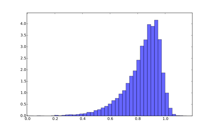
To illustrate the bias in $\hat \beta$, listing 10 generates the data 10,000 times, computes $\hat \beta$ on each occasion and histograms the result. The parameters are $N = 25$ and $\beta = 0.9$. The output is figure 12.4. If you modify the code to print the sample mean, it gives around 0.82. Since the number of replications is large, this is close to $\EE[\hat \beta]$. An asymptotic 95% confidence interval for our estimate is around (0.818, 0.824).

import numpy as np
import matplotlib.pyplot as plt

N = 25
x = np.zeros(N)
beta = 0.9                    
num_reps = 10000               
betahat_obs = np.empty(num_reps)
                        
for j in range(num_reps):
    u = np.random.randn(N)
    for t in range(N-1):
        x[t+1] = beta * x[t] + u[t+1]
    y = x[1:]       # x_1 ,..., x_N          
    x_vec = x[:-1]  # x_0, ..., x_{N-1}
    betahat_obs[j]  = np.sum(x_vec * y) / np.sum(x_vec**2)

plt.hist(betahat_obs, bins=50, alpha=0.6, density=True)
plt.show()

12.2.3Instrumental Variables¶

The discussion in Section 12.2.2 shows that the OLS estimator is biased and inconsistent when regressors are endogenous. Here we show that a consistent estimator of $\boldbeta$ can be found when extra information is available in the form of "exogenous" variables called instruments. These instruments will be collected into a $N \times J$ matrix $\boldZ$, where each column is observations on one exogenous variable. We connect $\boldZ$ and the other variables via the following assumptions:

As exercise 12.4.18 asks you to show, assumption (iv) implies that $J \geq K$, which is to say that we have at least as many instruments as regressors. If $J > K$, the model is said to be overidentified. If $J=K$, the model is called exactly identified. (When $J < K$, the model is called underidentified.)

The idea of instrumental variables least squares is to multiply $\boldy = \boldX \boldbeta + \boldu$ by $\boldZ^\T$ to produce

Applying (ii) and (iii) from the IV assumptions gives $\EE[ \boldw \given \boldZ] = \boldzero$ and $\EE [ \boldw \boldw^\T \given \boldZ] = \sigma^2 \boldZ^\T \boldZ$. This suggests that we might apply generalized least squares estimation to the linear equation in (12.32). We can use the expression for the GLS estimator from (12.27) after substituting $\boldX$ for $\boldZ^\T \boldX$, $\boldy$ for $\boldZ^\T \boldy$, and $\boldOmega$ for $\sigma^2 \boldZ^\T \boldZ$. This leads to the instrumental variable least squares (IVLS) estimator

In the case where $J = K$, this reduces to the simpler expression

In the preceding discussion, the analogy with GLS was not exact. (Direct application of GLS to (12.32) would require that $\EE[ \boldw \given \boldZ^\T \boldX] = \boldzero$ rather than $\EE[ \boldw \given \boldZ] = \boldzero$.) As a consequence we cannot claim unbiasedness and other properties by appealing to the GLS theory. Indeed $\hboldbeta_{{\rm IVLS}}$ is, in general, biased (see ex. 12.4.20).

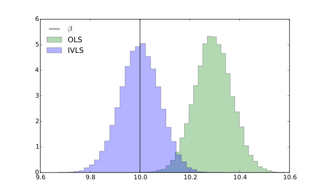
At the same time, the bias is typically smaller than OLS and vanishes asymptotically (see, e.g., §8.3 of Davidson & MacKinnon (2004)). Figure 12.5 gives an illustration. This figure corresponds to OLS and IVLS estimates of $\beta$ in $y = x \beta + u$ when $\beta=10$, $z$ is drawn independently of $u$, and $x$ is set equal to $\alpha z + (1 - \alpha) u$. Thus $z$ is exogenous and $x$ is a mixture of $z$ and $u$. The value $\alpha$ is a constant. In the simulation, $\alpha$ is set to $0.8$, so $z$ is a relatively strong instrument. The histograms are observations of the two estimators over 25,000 repetitions, each one having a sample size of $250$. IV provides a much better estimator of $\beta$ in this case.

There is another way to derive the expression given for $\hboldbeta_{{\rm IVLS}}$ on the right-hand side of (12.33). It involves a method called two-stage least squares. The key idea is to project the endogenous regressors onto the column space of the exogenous instruments before running the regression. Exercise 12.4.21 walks you through the details.

12.2.4Causality¶

Causality is a slippery concept. Let’s touch on some basic points, particularly concerning the connection between causality and regression. (References to more detailed treatments are given in Section 12.3.)

You might have heard $R^2$ interpreted as measuring the “explanatory power” of the regressors in a particular econometric problem. The idea is that regression amounts to decomposing $\boldy$ into the sum of two orthogonal parts, the fitted values $\boldP \boldy$ and the residuals $\boldM \boldy$. As in (11.12), the squared norm $\| \boldy\|^2 =: \tss$ can then be decomposed as $\| \boldP \boldy\|^2 =: \ess$ plus $\| \boldM \boldy\|^2 =: \rss$. This is sometimes paraphrased as “the total variation in $\boldy$ is the sum of explained and unexplained variation.” The value of $R^2$ is then claimed to be the fraction of the variation in $\boldy$ “explained” by the regressors.

This terminology is problematic because the notion that the regressors “explain” variation in $\boldy$ suggests causation, and $R^2$ says nothing about causation per se. Instead, $R^2$ is better thought of as a measure of correlation (see Section 11.2.3). As has been observed on many occasions, correlation and causation are not the same thing. Two informal examples are as follows:

• We often see car crashes and ambulances together (correlation). This does not imply that ambulances cause crashes.

• Say we observe that people sleeping with their shoes on often wake up with sore heads. One possible explanation is that wearing shoes to bed causes headaches. Another is that both phenomena are caused by too many pints at the pub the night before.

Identifying causality in observational data can be very challenging. Here’s another example, which, although it falls in the realm of traffic safety, is nonetheless interesting because it involves choices and human behavior: It has been observed that motorcycles fitted with ABS brakes have much lower crash rates than those without anti-lock brakes (see, e.g., Teoh (2011)). Does that mean fitting ABS to a given motorcycle will reduce the probability that the bike is involved in an accident by a similar amount? If so, should traffic authorities mandate the use of ABS brakes?

There’s an obvious problem in jumping to this conclusion: selection bias in the sample. Cautious motorcyclists are more likely to choose bikes with safety features such as ABS. Lower crash rates for ABS bikes might therefore be caused primarily by more careful riding.

We can eliminate the selection bias by randomly assigning bikes of both types to a large group of riders and observing the results. One might expect that such randomization would reduce the observed effect, although perhaps not eliminate it entirely. In fact such a study has already been conducted for the case of passenger vehicles. In Munich, half of a large fleet of taxis were fitted with anti-lock brakes and half were fitted with conventional brakes (Aschenbrenner & Biehl (1994)). The study lasted three years and drivers were randomly assigned across vehicles. A total of 747 accidents were observed. The authors found that accidents rates where slightly higher for taxis fitted with ABS.

The conclusion of the authors is that, while anti-lock brakes do improve braking performance, drivers compensate by driving faster, making shaper turns, poorer lane changes, and so forth. (This altered behavior is called "risk compensation.") The net effect is roughly zero: mandatory ABS brakes will cause no appreciable drop in accident rates.

In general, understanding causality requires either good experiments or good theory. There is no magic econometric procedure that can reliably extract causality from observational data without a good model.

12.3Further Reading¶

General econometrics texts treating OLS and its extensions include Hayashi (2000), Kennedy (2008), Greene (2011), Davidson & MacKinnon (2004), Wooldridge (2010), and Cameron & Trivedi (2005). A comprehensive treatment of theory can be found in Ruud (2000).

Regarding robust standard errors, asymptotics of the estimator in (12.28) are provided in White (1980). Closely related is the covariance matrix estimator proposed in Newey & West (1987). See Hayashi (2000), Hansen (2015), and Cameron & Trivedi (2005) for textbook treatments.

Measurement errors form another source of bias in OLS estimators. There is a standard approach to so-called errors-in-variables models based around instrumental variables. See, for example, chapter 8 of Davidson & MacKinnon (2004). For a treatment of nonlinear errors-in-variables, see Chen et al. (2011).

For more discussion of causality, see Freedman (2009), Angrist & Pischke (2009), Pearl (2009), or Imbens & Rubin (2015). An important notion of causality in time series models is the ability of one time series to predict another. A seminal contribution is Granger (1969). See Dufour & Taamouti (2010) for a more recent discussion. Chernozhukov et al. (2013) consider how to perform inference on counterfactual distributions. Belloni et al. (2014) discuss treatment effects in high dimensional settings.

12.4Exercises¶

12.4.1Solutions to Selected Exercises¶