Chapter 5: Markov Decision Processes

inventory_dp.jl

include("s_approx.jl")
using Distributions
m(x) = max(x, 0)  # Convenience function

function create_inventory_model(; β=0.98,     # discount factor
                                  K=40,       # maximum inventory
                                  c=0.2, κ=2, # cost paramters
                                  p=0.6)      # demand parameter
    ϕ(d) = (1 - p)^d * p        # demand pdf
    x_vals = collect(0:K)       # set of inventory levels
    return (; β, K, c, κ, p, ϕ, x_vals)
end

"The function B(x, a, v) = r(x, a) + β Σ_x′ v(x′) P(x, a, x′)."
function B(x, a, v, model; d_max=100)
    (; β, K, c, κ, p, ϕ, x_vals) = model
    revenue = sum(min(x, d) * ϕ(d) for d in 0:d_max) 
    current_profit = revenue - c * a - κ * (a > 0)
    next_value = sum(v[m(x - d) + a + 1] * ϕ(d) for d in 0:d_max)
    return current_profit + β * next_value
end

"The Bellman operator."
function T(v, model)
    (; β, K, c, κ, p, ϕ, x_vals) = model
    new_v = similar(v)
    for (x_idx, x) in enumerate(x_vals)
        Γx = 0:(K - x) 
        new_v[x_idx], _ = findmax(B(x, a, v, model) for a in Γx)
    end
    return new_v
end

"Get a v-greedy policy.  Returns a zero-based array."
function get_greedy(v, model)
    (; β, K, c, κ, p, ϕ, x_vals) = model
    σ_star = zero(x_vals)
    for (x_idx, x) in enumerate(x_vals)
        Γx = 0:(K - x) 
        _, a_idx = findmax(B(x, a, v, model) for a in Γx)
        σ_star[x_idx] = Γx[a_idx]
    end
    return σ_star
end

"Use successive_approx to get v_star and then compute greedy."
function solve_inventory_model(v_init, model)
    (; β, K, c, κ, p, ϕ, x_vals) = model
    v_star = successive_approx(v -> T(v, model), v_init)
    σ_star = get_greedy(v_star, model)
    return v_star, σ_star
end

# == Plots == # 

using PyPlot
using PyPlot
using LaTeXStrings
PyPlot.matplotlib[:rc]("text", usetex=true) # allow tex rendering

# Create an instance of the model and solve it
model = create_inventory_model()
(; β, K, c, κ, p, ϕ, x_vals) = model
v_init = zeros(length(x_vals))
v_star, σ_star = solve_inventory_model(v_init, model)

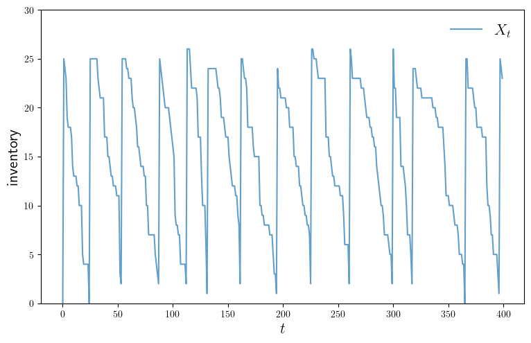
"Simulate given the optimal policy."
function sim_inventories(ts_length=400, X_init=0)
    G = Geometric(p)
    X = zeros(Int32, ts_length)
    X[1] = X_init
    for t in 1:(ts_length-1)
        D = rand(G)
        X[t+1] = m(X[t] - D) + σ_star[X[t] + 1]
    end
    return X
end


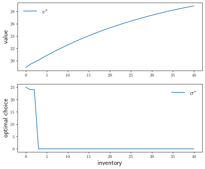
function plot_vstar_and_opt_policy(; fontsize=16, 
                   figname="./figures/inventory_dp_vs.pdf",
                   savefig=false)
    fig, axes = plt.subplots(2, 1, figsize=(8, 6.5))

    ax = axes[1]
    ax.plot(0:K, v_star, label=L"v^*")
    ax.set_ylabel("value", fontsize=fontsize)
    ax.legend(fontsize=fontsize, frameon=false)

    ax = axes[2]
    ax.plot(0:K, σ_star, label=L"\sigma^*")
    ax.set_xlabel("inventory", fontsize=fontsize)
    ax.set_ylabel("optimal choice", fontsize=fontsize)
    ax.legend(fontsize=fontsize, frameon=false)
    if savefig == true
        fig.savefig(figname)
    end
end

function plot_ts(; fontsize=16, 
                   figname="./figures/inventory_dp_ts.pdf",
                   savefig=false)
    X = sim_inventories()
    fig, ax = plt.subplots(figsize=(9, 5.5))
    ax.plot(X, label=L"X_t", alpha=0.7)
    ax.set_xlabel(L"t", fontsize=fontsize)
    ax.set_ylabel("inventory", fontsize=fontsize)
    ax.legend(fontsize=fontsize, frameon=false)
    ax.set_ylim(0, maximum(X)+4)
    if savefig == true
        fig.savefig(figname)
    end
end

Completed iteration 25 with error 0.41042666932980687.
Completed iteration 50 with error 0.21020630773590554.

Completed iteration 75 with error 0.0955793466139987.
Completed iteration 100 with error 0.057146989183511465.

Completed iteration 125 with error 0.03436202542500766.
Completed iteration 150 with error 0.020703850094779597.

Completed iteration 175 with error 0.012485135075589682.
Completed iteration 200 with error 0.007532190047619736.

Completed iteration 225 with error 0.004544855368770584.
Completed iteration 250 with error 0.0027425060040116023.

Completed iteration 275 with error 0.0016549687240292599.
Completed iteration 300 with error 0.0009987055387483679.

Completed iteration 325 with error 0.0006026809169377145.
Completed iteration 350 with error 0.0003636960443387238.

Completed iteration 375 with error 0.00021947756642148875.
Completed iteration 400 with error 0.00013244692466685137.

Completed iteration 425 with error 7.992703666204193e-5.
Completed iteration 450 with error 4.823314469604156e-5.

Completed iteration 475 with error 2.9107000830919105e-5.
Completed iteration 500 with error 1.7565048199941202e-5.

Completed iteration 525 with error 1.0599887019679954e-5.
Completed iteration 550 with error 6.396657951768248e-6.

Completed iteration 575 with error 3.860157463009273e-6.
Completed iteration 600 with error 2.3294688880071135e-6.

Completed iteration 625 with error 1.4057523145538653e-6.
Terminated successfully in 643 iterations.

plot_ts (generic function with 1 method)

plot_vstar_and_opt_policy(savefig=true)

plot_ts(savefig=true)

finite_opt_saving_0.jl

using QuantEcon, LinearAlgebra, IterTools

function create_savings_model(; R=1.01, β=0.98, γ=2.5,  
                                w_min=0.01, w_max=20.0, w_size=200,
                                ρ=0.9, ν=0.1, y_size=5)
    w_grid = LinRange(w_min, w_max, w_size)  
    mc = tauchen(y_size, ρ, ν)
    y_grid, Q = exp.(mc.state_values), mc.p
    return (; β, R, γ, w_grid, y_grid, Q)
end

"B(w, y, w′, v) = u(R*w + y - w′) + β Σ_y′ v(w′, y′) Q(y, y′)."
function B(i, j, k, v, model)
    (; β, R, γ, w_grid, y_grid, Q) = model
    w, y, w′ = w_grid[i], y_grid[j], w_grid[k]
    u(c) = c^(1-γ) / (1-γ)
    c = w + y - (w′ / R)
    @views value = c > 0 ? u(c) + β * dot(v[k, :], Q[j, :]) : -Inf
    return value
end

"The Bellman operator."
function T(v, model)
    w_idx, y_idx = (eachindex(g) for g in (model.w_grid, model.y_grid))
    v_new = similar(v)
    for (i, j) in product(w_idx, y_idx)
        v_new[i, j] = maximum(B(i, j, k, v, model) for k in w_idx)
    end
    return v_new
end

"The policy operator."
function T_σ(v, σ, model)
    w_idx, y_idx = (eachindex(g) for g in (model.w_grid, model.y_grid))
    v_new = similar(v)
    for (i, j) in product(w_idx, y_idx)
        v_new[i, j] = B(i, j, σ[i, j], v, model) 
    end
    return v_new
end

T_σ

finite_opt_saving_1.jl

include("finite_opt_saving_0.jl")

"Compute a v-greedy policy."
function get_greedy(v, model)
    w_idx, y_idx = (eachindex(g) for g in (model.w_grid, model.y_grid))
    σ = Matrix{Int32}(undef, length(w_idx), length(y_idx))
    for (i, j) in product(w_idx, y_idx)
        _, σ[i, j] = findmax(B(i, j, k, v, model) for k in w_idx)
    end
    return σ
end

"Get the value v_σ of policy σ."
function get_value(σ, model)
    # Unpack and set up
    (; β, R, γ, w_grid, y_grid, Q) = model
    w_idx, y_idx = (eachindex(g) for g in (w_grid, y_grid))
    wn, yn = length(w_idx), length(y_idx)
    n = wn * yn
    u(c) = c^(1-γ) / (1-γ)
    # Build P_σ and r_σ as multi-index arrays
    P_σ = zeros(wn, yn, wn, yn)
    r_σ = zeros(wn, yn)
    for (i, j) in product(w_idx, y_idx)
            w, y, w′ = w_grid[i], y_grid[j], w_grid[σ[i, j]]
            r_σ[i, j] = u(w + y - w′/R)
        for (i′, j′) in product(w_idx, y_idx)
            if i′ == σ[i, j]
                P_σ[i, j, i′, j′] = Q[j, j′]
            end
        end
    end
    # Reshape for matrix algebra
    P_σ = reshape(P_σ, n, n)
    r_σ = reshape(r_σ, n)
    # Apply matrix operations --- solve for the value of σ 
    v_σ = (I - β * P_σ) \ r_σ
    # Return as multi-index array
    return reshape(v_σ, wn, yn)
end

get_value

finite_opt_saving_2.jl

include("s_approx.jl")
include("finite_opt_saving_1.jl")

"Value function iteration routine."
function value_iteration(model, tol=1e-5)
    vz = zeros(length(model.w_grid), length(model.y_grid))
    v_star = successive_approx(v -> T(v, model), vz, tolerance=tol)
    return get_greedy(v_star, model)
end

"Howard policy iteration routine."
function policy_iteration(model)
    wn, yn = length(model.w_grid), length(model.y_grid)
    σ = ones(Int32, wn, yn)
    i, error = 0, 1.0
    while error > 0
        v_σ = get_value(σ, model)
        σ_new = get_greedy(v_σ, model)
        error = maximum(abs.(σ_new - σ))
        σ = σ_new
        i = i + 1
        println("Concluded loop $i with error $error.")
    end
    return σ
end

"Optimistic policy iteration routine."
function optimistic_policy_iteration(model; tolerance=1e-5, m=100)
    v = zeros(length(model.w_grid), length(model.y_grid))
    error = tolerance + 1
    while error > tolerance
        last_v = v
        σ = get_greedy(v, model)
        for i in 1:m
            v = T_σ(v, σ, model)
        end
        error = maximum(abs.(v - last_v))
    end
    return get_greedy(v, model)
end

# == Simulations and inequality measures == #

function simulate_wealth(m)

    model = create_savings_model()
    σ_star = optimistic_policy_iteration(model)
    (; β, R, γ, w_grid, y_grid, Q) = model

    # Simulate labor income (indices rather than grid values)
    mc = MarkovChain(Q)
    y_idx_series = simulate(mc, m)

    # Compute corresponding wealth time series
    w_idx_series = similar(y_idx_series)
    w_idx_series[1] = 1  # initial condition
    for t in 1:(m-1)
        i, j = w_idx_series[t], y_idx_series[t]
        w_idx_series[t+1] = σ_star[i, j]
    end
    w_series = w_grid[w_idx_series]

    return w_series
end

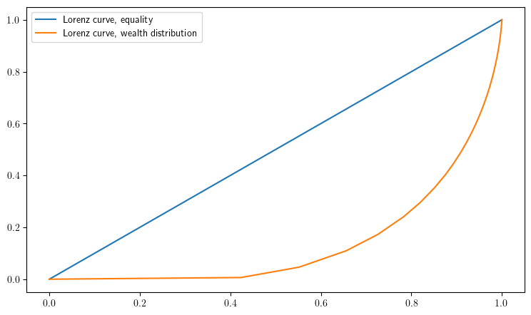
function lorenz(v)  # assumed sorted vector
    S = cumsum(v)  # cumulative sums: [v[1], v[1] + v[2], ... ]
    F = (1:length(v)) / length(v)
    L = S ./ S[end]
    return (; F, L) # returns named tuple
end

gini(v) = (2 * sum(i * y for (i,y) in enumerate(v))/sum(v)
           - (length(v) + 1))/length(v)



# == Plots == #

using PyPlot
using LaTeXStrings
PyPlot.matplotlib[:rc]("text", usetex=true) # allow tex rendering
fontsize=16

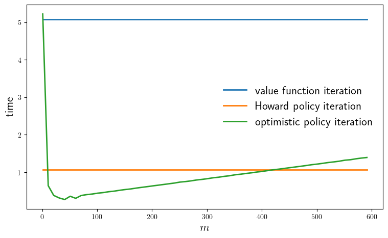
function plot_timing(; m_vals=collect(range(1, 600, step=10)),
                       savefig=false)
    model = create_savings_model(y_size=5)
    println("Running Howard policy iteration.")
    pi_time = @elapsed σ_pi = policy_iteration(model)
    println("PI completed in $pi_time seconds.")
    println("Running value function iteration.")
    vfi_time = @elapsed σ_vfi = value_iteration(model)
    println("VFI completed in $vfi_time seconds.")
    @assert σ_vfi == σ_pi "Warning: policies deviated."
    opi_times = []
    for m in m_vals
        println("Running optimistic policy iteration with m=$m.")
        opi_time = @elapsed σ_opi = optimistic_policy_iteration(model, m=m)
        @assert σ_opi == σ_pi "Warning: policies deviated."
        println("OPI with m=$m completed in $opi_time seconds.")
        push!(opi_times, opi_time)
    end
    fig, ax = plt.subplots(figsize=(9, 5.2))
    ax.plot(m_vals, fill(vfi_time, length(m_vals)), 
            lw=2, label="value function iteration")
    ax.plot(m_vals, fill(pi_time, length(m_vals)), 
            lw=2, label="Howard policy iteration")
    ax.plot(m_vals, opi_times, lw=2, label="optimistic policy iteration")
    ax.legend(fontsize=fontsize, frameon=false)
    ax.set_xlabel(L"m", fontsize=fontsize)
    ax.set_ylabel("time", fontsize=fontsize)
    if savefig
        fig.savefig("./figures/finite_opt_saving_2_1.pdf")
    end
    return (pi_time, vfi_time, opi_times)
end

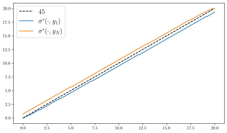
function plot_policy(; method="pi")
    model = create_savings_model()
    (; β, R, γ, w_grid, y_grid, Q) = model
    if method == "vfi"
        σ_star =  value_iteration(model) 
    elseif method == "pi"
        σ_star = policy_iteration(model) 
    else
        σ_star = optimistic_policy_iteration(model)
    end
    fig, ax = plt.subplots(figsize=(9, 5.2))
    ax.plot(w_grid, w_grid, "k--", label=L"45")
    ax.plot(w_grid, w_grid[σ_star[:, 1]], label=L"\sigma^*(\cdot, y_1)")
    ax.plot(w_grid, w_grid[σ_star[:, end]], label=L"\sigma^*(\cdot, y_N)")
    ax.legend(fontsize=fontsize)
end


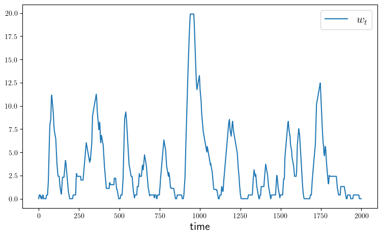
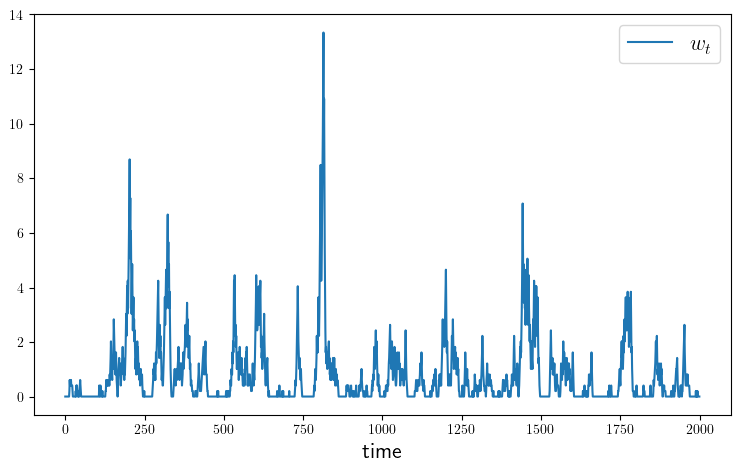
function plot_time_series(; m=2_000,
                           savefig=false, 
                           figname="./figures/finite_opt_saving_ts.pdf")

    w_series = simulate_wealth(m)
    fig, ax = plt.subplots(figsize=(9, 5.2))
    ax.plot(w_series, label=L"w_t")
    ax.set_xlabel("time", fontsize=fontsize)
    ax.legend(fontsize=fontsize)
    if savefig
        fig.savefig(figname)
    end
end

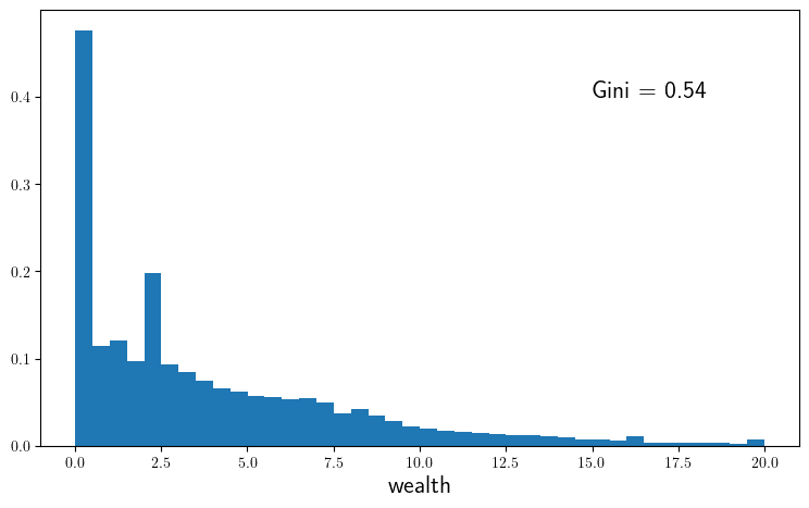
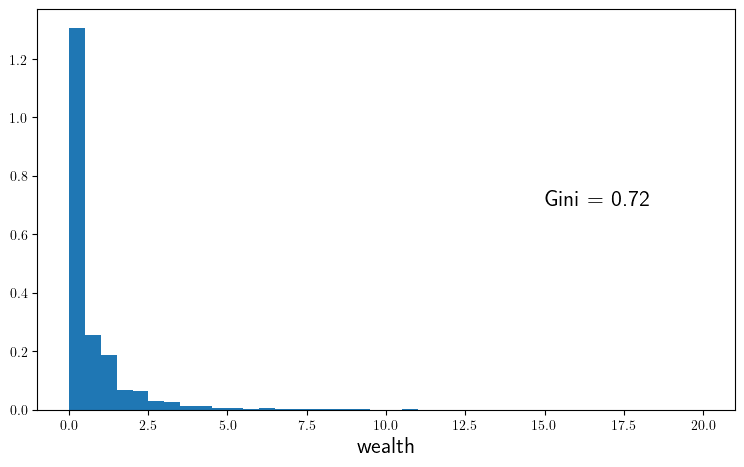
function plot_histogram(; m=1_000_000,
                           savefig=false, 
                           figname="./figures/finite_opt_saving_hist.pdf")

    w_series = simulate_wealth(m)
    g = round(gini(sort(w_series)), digits=2)
    fig, ax = plt.subplots(figsize=(9, 5.2))
    ax.hist(w_series, bins=40, density=true)
    ax.set_xlabel("wealth", fontsize=fontsize)
    ax.text(15, 0.4, "Gini = $g", fontsize=fontsize)

    if savefig
        fig.savefig(figname)
    end
end

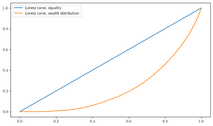
function plot_lorenz(; m=1_000_000,
                           savefig=false, 
                           figname="./figures/finite_opt_saving_lorenz.pdf")

    w_series = simulate_wealth(m)
    (; F, L) = lorenz(sort(w_series))

    fig, ax = plt.subplots(figsize=(9, 5.2))
    ax.plot(F, F, label="Lorenz curve, equality")
    ax.plot(F, L, label="Lorenz curve, wealth distribution")
    ax.legend()

    if savefig
        fig.savefig(figname)
    end
end

plot_lorenz (generic function with 1 method)

plot_timing(savefig=true)

Running Howard policy iteration.
Concluded loop 1 with error 100.

Concluded loop 2 with error 80.
Concluded loop 3 with error 34.

Concluded loop 4 with error 20.
Concluded loop 5 with error 11.
Concluded loop 6 with error 5.

Concluded loop 7 with error 5.
Concluded loop 8 with error 3.
Concluded loop 9 with error 1.

Concluded loop 10 with error 1.
Concluded loop 11 with error 1.
Concluded loop 12 with error 1.

Concluded loop 13 with error 1.
Concluded loop 14 with error 1.
Concluded loop 15 with error 1.

Concluded loop 16 with error 1.
Concluded loop 17 with error 1.
Concluded loop 18 with error 1.

Concluded loop 19 with error 1.
Concluded loop 20 with error 1.
Concluded loop 21 with error 1.

Concluded loop 22 with error 1.
Concluded loop 23 with error 1.
Concluded loop 24 with error 0.
PI completed in 1.071244493 seconds.
Running value function iteration.

Completed iteration 25 with error 0.536460823305255.

Completed iteration 50 with error 0.2757145835707817.

Completed iteration 75 with error 0.15964723339325104.

Completed iteration 100 with error 0.0949415406202192.

Completed iteration 125 with error 0.056923225476566586.

Completed iteration 150 with error 0.034240232785961666.

Completed iteration 175 with error 0.02062794785982902.

Completed iteration 200 with error 0.012437154854261223.

Completed iteration 225 with error 0.007501837673252965.

Completed iteration 250 with error 0.004525955103851231.

Completed iteration 275 with error 0.0027308880659973056.

Completed iteration 300 with error 0.0016478769789074477.

Completed iteration 325 with error 0.0009943978415378751.

Completed iteration 350 with error 0.0006000718833263363.

Completed iteration 375 with error 0.000362118316374449.

Completed iteration 400 with error 0.00021852437882330378.

Completed iteration 425 with error 0.00013187135264303151.

Completed iteration 450 with error 7.957958084148231e-5.

Completed iteration 475 with error 4.802342870391385e-5.

Completed iteration 500 with error 2.8980432084324548e-5.

Completed iteration 525 with error 1.7488664326492653e-5.

Completed iteration 550 with error 1.0553790723122347e-5.
Terminated successfully in 554 iterations.
VFI completed in 5.074801232 seconds.
Running optimistic policy iteration with m=1.

OPI with m=1 completed in 5.221025954 seconds.
Running optimistic policy iteration with m=11.

OPI with m=11 completed in 0.642277183 seconds.
Running optimistic policy iteration with m=21.

OPI with m=21 completed in 0.38293115 seconds.
Running optimistic policy iteration with m=31.

OPI with m=31 completed in 0.315024091 seconds.
Running optimistic policy iteration with m=41.

OPI with m=41 completed in 0.272764744 seconds.
Running optimistic policy iteration with m=51.

OPI with m=51 completed in 0.360400965 seconds.
Running optimistic policy iteration with m=61.

OPI with m=61 completed in 0.30517861 seconds.
Running optimistic policy iteration with m=71.

OPI with m=71 completed in 0.380866333 seconds.
Running optimistic policy iteration with m=81.

OPI with m=81 completed in 0.403981523 seconds.
Running optimistic policy iteration with m=91.

OPI with m=91 completed in 0.419655452 seconds.
Running optimistic policy iteration with m=101.

OPI with m=101 completed in 0.442634941 seconds.
Running optimistic policy iteration with m=111.

OPI with m=111 completed in 0.458257969 seconds.
Running optimistic policy iteration with m=121.

OPI with m=121 completed in 0.48136366 seconds.
Running optimistic policy iteration with m=131.

OPI with m=131 completed in 0.496775186 seconds.
Running optimistic policy iteration with m=141.

OPI with m=141 completed in 0.519935477 seconds.
Running optimistic policy iteration with m=151.

OPI with m=151 completed in 0.539455357 seconds.
Running optimistic policy iteration with m=161.

OPI with m=161 completed in 0.555373837 seconds.
Running optimistic policy iteration with m=171.

OPI with m=171 completed in 0.57793703 seconds.
Running optimistic policy iteration with m=181.

OPI with m=181 completed in 0.597732298 seconds.
Running optimistic policy iteration with m=191.

OPI with m=191 completed in 0.616370657 seconds.
Running optimistic policy iteration with m=201.

OPI with m=201 completed in 0.63653003 seconds.
Running optimistic policy iteration with m=211.

OPI with m=211 completed in 0.65537379 seconds.
Running optimistic policy iteration with m=221.

OPI with m=221 completed in 0.674622254 seconds.
Running optimistic policy iteration with m=231.

OPI with m=231 completed in 0.693936019 seconds.
Running optimistic policy iteration with m=241.

OPI with m=241 completed in 0.713445685 seconds.
Running optimistic policy iteration with m=251.

OPI with m=251 completed in 0.738912803 seconds.
Running optimistic policy iteration with m=261.

OPI with m=261 completed in 0.752197216 seconds.
Running optimistic policy iteration with m=271.

OPI with m=271 completed in 0.771088148 seconds.
Running optimistic policy iteration with m=281.

OPI with m=281 completed in 0.794194224 seconds.
Running optimistic policy iteration with m=291.

OPI with m=291 completed in 0.810279188 seconds.
Running optimistic policy iteration with m=301.

OPI with m=301 completed in 0.829489085 seconds.
Running optimistic policy iteration with m=311.

OPI with m=311 completed in 0.852653222 seconds.
Running optimistic policy iteration with m=321.

OPI with m=321 completed in 0.868018179 seconds.
Running optimistic policy iteration with m=331.

OPI with m=331 completed in 0.89044751 seconds.
Running optimistic policy iteration with m=341.

OPI with m=341 completed in 0.907291626 seconds.
Running optimistic policy iteration with m=351.

OPI with m=351 completed in 0.932635328 seconds.
Running optimistic policy iteration with m=361.

OPI with m=361 completed in 0.948747957 seconds.
Running optimistic policy iteration with m=371.

OPI with m=371 completed in 0.967916864 seconds.
Running optimistic policy iteration with m=381.

OPI with m=381 completed in 0.986039319 seconds.
Running optimistic policy iteration with m=391.

OPI with m=391 completed in 1.007013186 seconds.
Running optimistic policy iteration with m=401.

OPI with m=401 completed in 1.023575619 seconds.
Running optimistic policy iteration with m=411.

OPI with m=411 completed in 1.045962499 seconds.
Running optimistic policy iteration with m=421.

OPI with m=421 completed in 1.067738275 seconds.
Running optimistic policy iteration with m=431.

OPI with m=431 completed in 1.084070205 seconds.
Running optimistic policy iteration with m=441.

OPI with m=441 completed in 1.103835279 seconds.
Running optimistic policy iteration with m=451.

OPI with m=451 completed in 1.123038341 seconds.
Running optimistic policy iteration with m=461.

OPI with m=461 completed in 1.142236397 seconds.
Running optimistic policy iteration with m=471.

OPI with m=471 completed in 1.16101795 seconds.
Running optimistic policy iteration with m=481.

OPI with m=481 completed in 1.181045213 seconds.
Running optimistic policy iteration with m=491.

OPI with m=491 completed in 1.203013892 seconds.
Running optimistic policy iteration with m=501.

OPI with m=501 completed in 1.219454626 seconds.
Running optimistic policy iteration with m=511.

OPI with m=511 completed in 1.239470452 seconds.
Running optimistic policy iteration with m=521.

OPI with m=521 completed in 1.260863948 seconds.
Running optimistic policy iteration with m=531.

OPI with m=531 completed in 1.277141179 seconds.
Running optimistic policy iteration with m=541.

OPI with m=541 completed in 1.296208832 seconds.
Running optimistic policy iteration with m=551.

OPI with m=551 completed in 1.322352843 seconds.
Running optimistic policy iteration with m=561.

OPI with m=561 completed in 1.334733542 seconds.
Running optimistic policy iteration with m=571.

OPI with m=571 completed in 1.359200363 seconds.
Running optimistic policy iteration with m=581.

OPI with m=581 completed in 1.378981331 seconds.
Running optimistic policy iteration with m=591.

OPI with m=591 completed in 1.394128555 seconds.

(1.071244493, 5.074801232, Any[5.221025954, 0.642277183, 0.38293115, 0.315024091, 0.272764744, 0.360400965, 0.30517861, 0.380866333, 0.403981523, 0.419655452  …  1.219454626, 1.239470452, 1.260863948, 1.277141179, 1.296208832, 1.322352843, 1.334733542, 1.359200363, 1.378981331, 1.394128555])

plot_policy()

Concluded loop 1 with error 100.
Concluded loop 2 with error 80.

Concluded loop 3 with error 34.
Concluded loop 4 with error 20.
Concluded loop 5 with error 11.

Concluded loop 6 with error 5.
Concluded loop 7 with error 5.
Concluded loop 8 with error 3.

Concluded loop 9 with error 1.
Concluded loop 10 with error 1.
Concluded loop 11 with error 1.

Concluded loop 12 with error 1.
Concluded loop 13 with error 1.
Concluded loop 14 with error 1.

Concluded loop 15 with error 1.
Concluded loop 16 with error 1.
Concluded loop 17 with error 1.

Concluded loop 18 with error 1.
Concluded loop 19 with error 1.
Concluded loop 20 with error 1.

Concluded loop 21 with error 1.
Concluded loop 22 with error 1.
Concluded loop 23 with error 1.

Concluded loop 24 with error 0.

PyObject <matplotlib.legend.Legend object at 0x7ffa448f6050>

plot_time_series(savefig=true)

plot_histogram(savefig=true)

plot_lorenz(savefig=true)

finite_lq.jl

using QuantEcon, LinearAlgebra, IterTools
include("s_approx.jl")

function create_investment_model(; 
        r=0.04,                              # Interest rate
        a_0=10.0, a_1=1.0,                   # Demand parameters
        γ=25.0, c=1.0,                       # Adjustment and unit cost 
        y_min=0.0, y_max=20.0, y_size=100,   # Grid for output
        ρ=0.9, ν=1.0,                        # AR(1) parameters
        z_size=25)                           # Grid size for shock
    β = 1/(1+r) 
    y_grid = LinRange(y_min, y_max, y_size)  
    mc = tauchen(y_size, ρ, ν)
    z_grid, Q = mc.state_values, mc.p
    return (; β, a_0, a_1, γ, c, y_grid, z_grid, Q)
end

"""
The aggregator B is given by 

    B(y, z, y′) = r(y, z, y′) + β Σ_z′ v(y′, z′) Q(z, z′)."

where 

    r(y, z, y′) := (a_0 - a_1 * y + z - c) y - γ * (y′ - y)^2

"""
function B(i, j, k, v, model)
    (; β, a_0, a_1, γ, c, y_grid, z_grid, Q) = model
    y, z, y′ = y_grid[i], z_grid[j], y_grid[k]
    r = (a_0 - a_1 * y + z - c) * y - γ * (y′ - y)^2
    return @views r + β * dot(v[k, :], Q[j, :]) 
end

"The policy operator."
function T_σ(v, σ, model)
    y_idx, z_idx = (eachindex(g) for g in (model.y_grid, model.z_grid))
    v_new = similar(v)
    for (i, j) in product(y_idx, z_idx)
        v_new[i, j] = B(i, j, σ[i, j], v, model) 
    end
    return v_new
end

"The Bellman operator."
function T(v, model)
    y_idx, z_idx = (eachindex(g) for g in (model.y_grid, model.z_grid))
    v_new = similar(v)
    for (i, j) in product(y_idx, z_idx)
        v_new[i, j] = maximum(B(i, j, k, v, model) for k in y_idx)
    end
    return v_new
end

"Compute a v-greedy policy."
function get_greedy(v, model)
    y_idx, z_idx = (eachindex(g) for g in (model.y_grid, model.z_grid))
    σ = Matrix{Int32}(undef, length(y_idx), length(z_idx))
    for (i, j) in product(y_idx, z_idx)
        _, σ[i, j] = findmax(B(i, j, k, v, model) for k in y_idx)
    end
    return σ
end

"Value function iteration routine."
function value_iteration(model; tol=1e-5)
    vz = zeros(length(model.y_grid), length(model.z_grid))
    v_star = successive_approx(v -> T(v, model), vz, tolerance=tol)
    return get_greedy(v_star, model)
end



"Get the value v_σ of policy σ."
function get_value(σ, model)
    # Unpack and set up
    (; β, a_0, a_1, γ, c, y_grid, z_grid, Q) = model
    yn, zn = length(y_grid), length(z_grid)
    n = yn * zn
    # Function to extract (i, j) from m = i + (j-1)*yn"
    single_to_multi(m) = (m-1)%yn + 1, div(m-1, yn) + 1
    # Allocate and create single index versions of P_σ and r_σ
    P_σ = zeros(n, n)
    r_σ = zeros(n)
    for m in 1:n
        i, j = single_to_multi(m)
        y, z, y′ = y_grid[i], z_grid[j], y_grid[σ[i, j]]
        r_σ[m] = (a_0 - a_1 * y + z - c) * y - γ * (y′ - y)^2
        for m′ in 1:n
            i′, j′ = single_to_multi(m′)
            if i′ == σ[i, j]
                P_σ[m, m′] = Q[j, j′]
            end
        end
    end
    # Solve for the value of σ 
    v_σ = (I - β * P_σ) \ r_σ
    # Return as multi-index array
    return reshape(v_σ, yn, zn)
end


"Howard policy iteration routine."
function policy_iteration(model)
    yn, zn = length(model.y_grid), length(model.z_grid)
    σ = ones(Int32, yn, zn)
    i, error = 0, 1.0
    while error > 0
        v_σ = get_value(σ, model)
        σ_new = get_greedy(v_σ, model)
        error = maximum(abs.(σ_new - σ))
        σ = σ_new
        i = i + 1
        println("Concluded loop $i with error $error.")
    end
    return σ
end

"Optimistic policy iteration routine."
function optimistic_policy_iteration(model; tol=1e-5, m=100)
    v = zeros(length(model.y_grid), length(model.z_grid))
    error = tol + 1
    while error > tol
        last_v = v
        σ = get_greedy(v, model)
        for i in 1:m
            v = T_σ(v, σ, model)
        end
        error = maximum(abs.(v - last_v))
    end
    return get_greedy(v, model)
end


# Plots

using PyPlot
using LaTeXStrings
PyPlot.matplotlib[:rc]("text", usetex=true) # allow tex rendering
fontsize=12

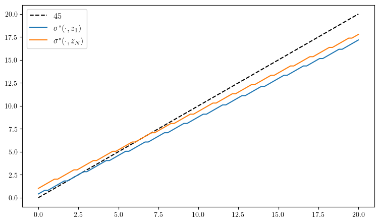
function plot_policy()
    model = create_investment_model()
    (; β, a_0, a_1, γ, c, y_grid, z_grid, Q) = model
    σ_star = optimistic_policy_iteration(model)
    fig, ax = plt.subplots(figsize=(9, 5.2))
    ax.plot(y_grid, y_grid, "k--", label=L"45")
    ax.plot(y_grid, y_grid[σ_star[:, 1]], label=L"\sigma^*(\cdot, z_1)")
    ax.plot(y_grid, y_grid[σ_star[:, end]], label=L"\sigma^*(\cdot, z_N)")
    ax.legend(fontsize=fontsize)
end

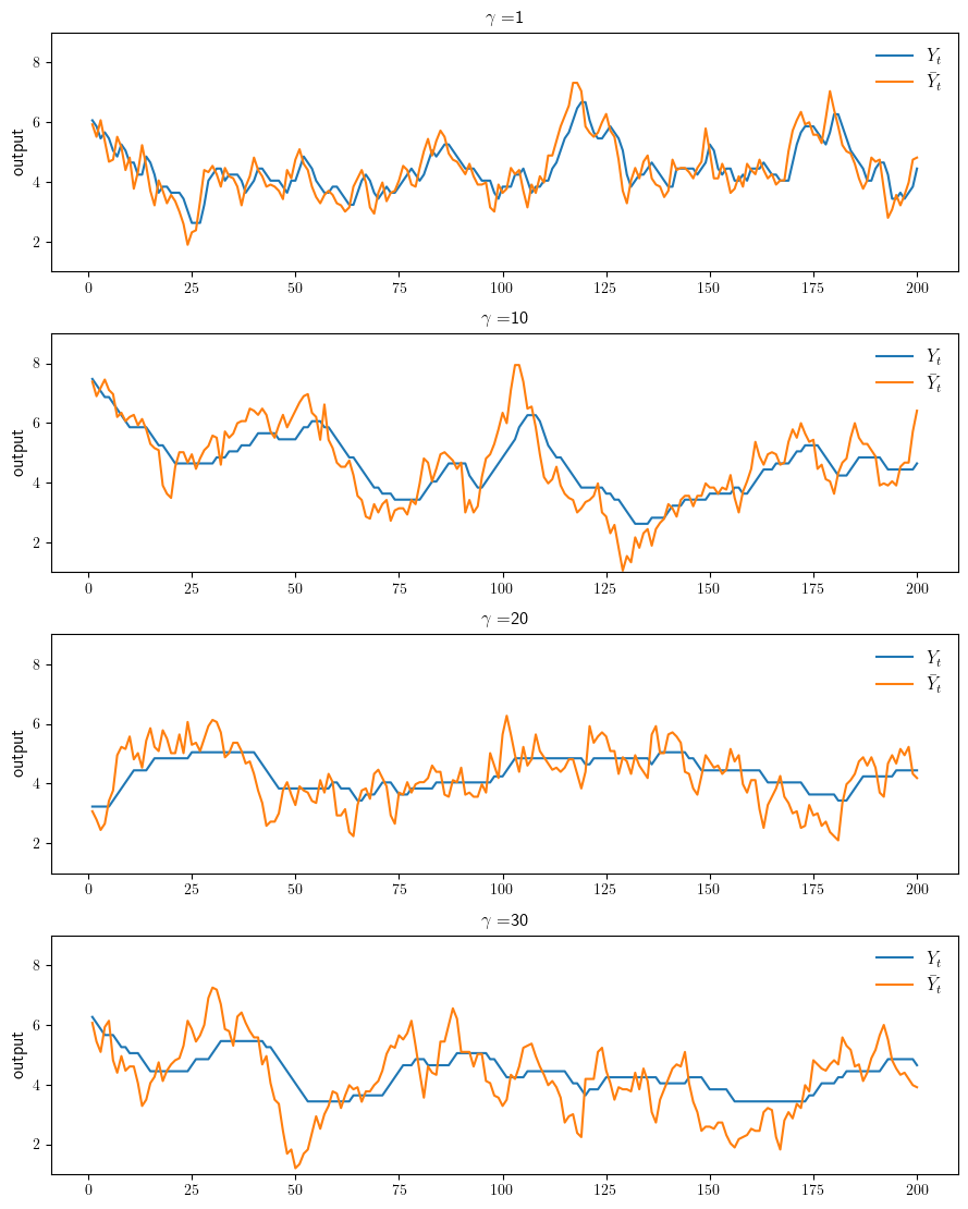
function plot_sim(; savefig=false, figname="./figures/finite_lq_1.pdf")
    ts_length = 200

    fig, axes = plt.subplots(4, 1, figsize=(9, 11.2))

    for (ax, γ) in zip(axes, (1, 10, 20, 30))
        model = create_investment_model(γ=γ)
        (; β, a_0, a_1, γ, c, y_grid, z_grid, Q) = model
        σ_star = optimistic_policy_iteration(model)
        mc = MarkovChain(Q, z_grid)

        z_sim_idx = simulate_indices(mc, ts_length)
        z_sim = z_grid[z_sim_idx]
        y_sim_idx = Vector{Int32}(undef, ts_length)
        y_1 = (a_0 - c + z_sim[1]) / (2 * a_1)
        y_sim_idx[1] = searchsortedfirst(y_grid, y_1)
        for t in 1:(ts_length-1)
            y_sim_idx[t+1] = σ_star[y_sim_idx[t], z_sim_idx[t]]
        end
        y_sim = y_grid[y_sim_idx]
        y_bar_sim = (a_0 .- c .+ z_sim) ./ (2 * a_1)

        ax.plot(1:ts_length, y_sim, label=L"Y_t")
        ax.plot(1:ts_length, y_bar_sim, label=L"\bar Y_t")
        ax.legend(fontsize=fontsize, frameon=false, loc="upper right")
        ax.set_ylabel("output", fontsize=fontsize)
        ax.set_ylim(1, 9)
        ax.set_title(L"\gamma = " * "$γ", fontsize=fontsize)
    end

    fig.tight_layout()
    if savefig
        fig.savefig(figname)
    end
end


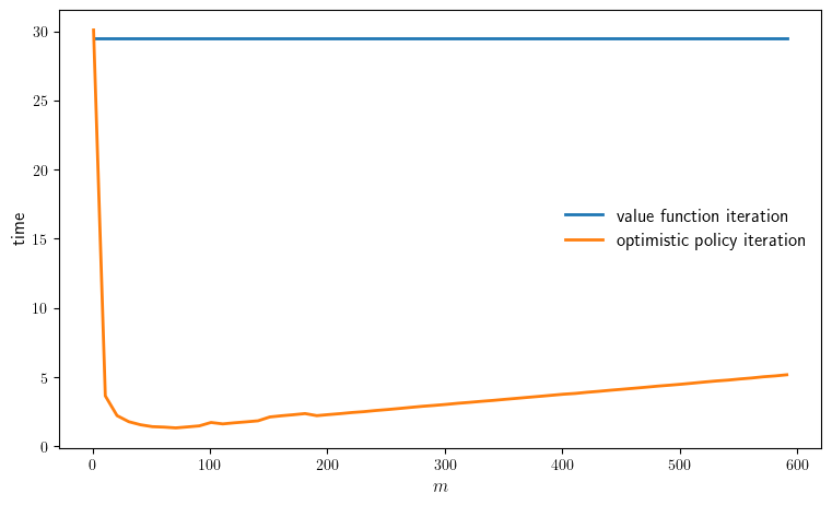
function plot_timing(; m_vals=collect(range(1, 600, step=10)),
                   savefig=false,
                   figname="./figures/finite_lq_time.pdf"
    )
    model = create_investment_model()
    #println("Running Howard policy iteration.")
    #pi_time = @elapsed σ_pi = policy_iteration(model)
    #println("PI completed in $pi_time seconds.")
    println("Running value function iteration.")
    vfi_time = @elapsed σ_vfi = value_iteration(model, tol=1e-5)
    println("VFI completed in $vfi_time seconds.")
    #@assert σ_vfi == σ_pi "Warning: policies deviated."
    opi_times = []
    for m in m_vals
        println("Running optimistic policy iteration with m=$m.")
        opi_time = @elapsed σ_opi = 
            optimistic_policy_iteration(model, m=m, tol=1e-5)
        println("OPI with m=$m completed in $opi_time seconds.")
        #@assert σ_opi == σ_pi "Warning: policies deviated."
        push!(opi_times, opi_time)
    end
    fig, ax = plt.subplots(figsize=(9, 5.2))
    #ax.plot(m_vals, fill(pi_time, length(m_vals)), 
    #        lw=2, label="Howard policy iteration")
    ax.plot(m_vals, fill(vfi_time, length(m_vals)), 
            lw=2, label="value function iteration")
    ax.plot(m_vals, opi_times, lw=2, label="optimistic policy iteration")
    ax.legend(fontsize=fontsize, frameon=false)
    ax.set_xlabel(L"m", fontsize=fontsize)
    ax.set_ylabel("time", fontsize=fontsize)
    if savefig
        fig.savefig(figname)
    end
    return (vfi_time, opi_times)
    #return (pi_time, vfi_time, opi_times)
end

plot_timing (generic function with 1 method)

plot_policy()

PyObject <matplotlib.legend.Legend object at 0x7ffa3cf225f0>

plot_sim(savefig=true)

plot_timing(savefig=true)

Running value function iteration.

Completed iteration 25 with error 8.945294734337608.

Completed iteration 50 with error 3.0402862553363548.

Completed iteration 75 with error 1.1324022887380352.

Completed iteration 100 with error 0.42457216331251857.

Completed iteration 125 with error 0.15925863812981333.

Completed iteration 150 with error 0.059740446974956285.

Completed iteration 175 with error 0.02240964166935555.

Completed iteration 200 with error 0.008406233024288667.

Completed iteration 225 with error 0.003153319248781372.

Completed iteration 250 with error 0.0011828630333639012.

Completed iteration 275 with error 0.000443711798880031.

Completed iteration 300 with error 0.000166443751368206.

Completed iteration 325 with error 6.243584800813551e-5.

Completed iteration 350 with error 2.3420735942636384e-5.

Terminated successfully in 373 iterations.
VFI completed in 29.528784254 seconds.
Running optimistic policy iteration with m=1.

OPI with m=1 completed in 30.095170343 seconds.
Running optimistic policy iteration with m=11.

OPI with m=11 completed in 3.641234111 seconds.
Running optimistic policy iteration with m=21.

OPI with m=21 completed in 2.212893573 seconds.
Running optimistic policy iteration with m=31.

OPI with m=31 completed in 1.77439615 seconds.
Running optimistic policy iteration with m=41.

OPI with m=41 completed in 1.552479619 seconds.
Running optimistic policy iteration with m=51.

OPI with m=51 completed in 1.417083582 seconds.
Running optimistic policy iteration with m=61.

OPI with m=61 completed in 1.383042195 seconds.
Running optimistic policy iteration with m=71.

OPI with m=71 completed in 1.326534742 seconds.
Running optimistic policy iteration with m=81.

OPI with m=81 completed in 1.398026415 seconds.
Running optimistic policy iteration with m=91.

OPI with m=91 completed in 1.472676214 seconds.
Running optimistic policy iteration with m=101.

OPI with m=101 completed in 1.718935814 seconds.
Running optimistic policy iteration with m=111.

OPI with m=111 completed in 1.614846258 seconds.
Running optimistic policy iteration with m=121.

OPI with m=121 completed in 1.696500293 seconds.
Running optimistic policy iteration with m=131.

OPI with m=131 completed in 1.764404221 seconds.
Running optimistic policy iteration with m=141.

OPI with m=141 completed in 1.839526805 seconds.
Running optimistic policy iteration with m=151.

OPI with m=151 completed in 2.115838776 seconds.
Running optimistic policy iteration with m=161.

OPI with m=161 completed in 2.204164313 seconds.
Running optimistic policy iteration with m=171.

OPI with m=171 completed in 2.27768488 seconds.
Running optimistic policy iteration with m=181.

OPI with m=181 completed in 2.361526188 seconds.
Running optimistic policy iteration with m=191.

OPI with m=191 completed in 2.211369529 seconds.
Running optimistic policy iteration with m=201.

OPI with m=201 completed in 2.288002702 seconds.
Running optimistic policy iteration with m=211.

OPI with m=211 completed in 2.358191326 seconds.
Running optimistic policy iteration with m=221.

OPI with m=221 completed in 2.438015942 seconds.
Running optimistic policy iteration with m=231.

OPI with m=231 completed in 2.500110902 seconds.
Running optimistic policy iteration with m=241.

OPI with m=241 completed in 2.583121534 seconds.
Running optimistic policy iteration with m=251.

OPI with m=251 completed in 2.652044881 seconds.
Running optimistic policy iteration with m=261.

OPI with m=261 completed in 2.728939228 seconds.
Running optimistic policy iteration with m=271.

OPI with m=271 completed in 2.810227245 seconds.
Running optimistic policy iteration with m=281.

OPI with m=281 completed in 2.888711541 seconds.
Running optimistic policy iteration with m=291.

OPI with m=291 completed in 2.952884176 seconds.
Running optimistic policy iteration with m=301.

OPI with m=301 completed in 3.0250701 seconds.
Running optimistic policy iteration with m=311.

OPI with m=311 completed in 3.105722434 seconds.
Running optimistic policy iteration with m=321.

OPI with m=321 completed in 3.172856224 seconds.
Running optimistic policy iteration with m=331.

OPI with m=331 completed in 3.247302513 seconds.
Running optimistic policy iteration with m=341.

OPI with m=341 completed in 3.313224778 seconds.
Running optimistic policy iteration with m=351.

OPI with m=351 completed in 3.390549156 seconds.
Running optimistic policy iteration with m=361.

OPI with m=361 completed in 3.463900036 seconds.
Running optimistic policy iteration with m=371.

OPI with m=371 completed in 3.538459878 seconds.
Running optimistic policy iteration with m=381.

OPI with m=381 completed in 3.610924076 seconds.
Running optimistic policy iteration with m=391.

OPI with m=391 completed in 3.686457797 seconds.
Running optimistic policy iteration with m=401.

OPI with m=401 completed in 3.762841576 seconds.
Running optimistic policy iteration with m=411.

OPI with m=411 completed in 3.818335252 seconds.
Running optimistic policy iteration with m=421.

OPI with m=421 completed in 3.90208728 seconds.
Running optimistic policy iteration with m=431.

OPI with m=431 completed in 3.971463168 seconds.
Running optimistic policy iteration with m=441.

OPI with m=441 completed in 4.050011214 seconds.
Running optimistic policy iteration with m=451.

OPI with m=451 completed in 4.121213671 seconds.
Running optimistic policy iteration with m=461.

OPI with m=461 completed in 4.192308673 seconds.
Running optimistic policy iteration with m=471.

OPI with m=471 completed in 4.267083899 seconds.
Running optimistic policy iteration with m=481.

OPI with m=481 completed in 4.346875111 seconds.
Running optimistic policy iteration with m=491.

OPI with m=491 completed in 4.412880865 seconds.
Running optimistic policy iteration with m=501.

OPI with m=501 completed in 4.484071705 seconds.
Running optimistic policy iteration with m=511.

OPI with m=511 completed in 4.563008908 seconds.
Running optimistic policy iteration with m=521.

OPI with m=521 completed in 4.644867485 seconds.
Running optimistic policy iteration with m=531.

OPI with m=531 completed in 4.719903651 seconds.
Running optimistic policy iteration with m=541.

OPI with m=541 completed in 4.781838985 seconds.
Running optimistic policy iteration with m=551.

OPI with m=551 completed in 4.863136503 seconds.
Running optimistic policy iteration with m=561.

OPI with m=561 completed in 4.932964649 seconds.
Running optimistic policy iteration with m=571.

OPI with m=571 completed in 5.021018989 seconds.
Running optimistic policy iteration with m=581.

OPI with m=581 completed in 5.084325612 seconds.
Running optimistic policy iteration with m=591.

OPI with m=591 completed in 5.167479718 seconds.

(29.528784254, Any[30.095170343, 3.641234111, 2.212893573, 1.77439615, 1.552479619, 1.417083582, 1.383042195, 1.326534742, 1.398026415, 1.472676214  …  4.484071705, 4.563008908, 4.644867485, 4.719903651, 4.781838985, 4.863136503, 4.932964649, 5.021018989, 5.084325612, 5.167479718])

firm_hiring.jl

using QuantEcon, LinearAlgebra, IterTools

function create_hiring_model(; 
        r=0.04,                              # Interest rate
        κ=1.0,                               # Adjustment cost 
        α=0.4,                               # Production parameter
        p=1.0, w=1.0,                        # Price and wage
        l_min=0.0, l_max=30.0, l_size=100,   # Grid for labor
        ρ=0.9, ν=0.4, b=1.0,                 # AR(1) parameters
        z_size=100)                          # Grid size for shock
    β = 1/(1+r) 
    l_grid = LinRange(l_min, l_max, l_size)  
    mc = tauchen(z_size, ρ, ν, b, 6)
    z_grid, Q = mc.state_values, mc.p
    return (; β, κ, α, p, w, l_grid, z_grid, Q)
end

"""
The aggregator B is given by 

    B(l, z, l′) = r(l, z, l′) + β Σ_z′ v(l′, z′) Q(z, z′)."

where 

    r(l, z, l′) := p * z * f(l) - w * l - κ 1{l != l′}

"""
function B(i, j, k, v, model)
    (; β, κ, α, p, w, l_grid, z_grid, Q) = model
    l, z, l′ = l_grid[i], z_grid[j], l_grid[k]
    r = p * z * l^α - w * l - κ * (l != l′)
    return @views r + β * dot(v[k, :], Q[j, :]) 
end


"The policy operator."
function T_σ(v, σ, model)
    l_idx, z_idx = (eachindex(g) for g in (model.l_grid, model.z_grid))
    v_new = similar(v)
    for (i, j) in product(l_idx, z_idx)
        v_new[i, j] = B(i, j, σ[i, j], v, model) 
    end
    return v_new
end

"Compute a v-greedy policy."
function get_greedy(v, model)
    (; β, κ, α, p, w, l_grid, z_grid, Q) = model
    l_idx, z_idx = (eachindex(g) for g in (model.l_grid, model.z_grid))
    σ = Matrix{Int32}(undef, length(l_idx), length(z_idx))
    for (i, j) in product(l_idx, z_idx)
        _, σ[i, j] = findmax(B(i, j, k, v, model) for k in l_idx)
    end
    return σ
end

"Optimistic policy iteration routine."
function optimistic_policy_iteration(model; tolerance=1e-5, m=100)
    v = zeros(length(model.l_grid), length(model.z_grid))
    error = tolerance + 1
    while error > tolerance
        last_v = v
        σ = get_greedy(v, model)
        for i in 1:m
            v = T_σ(v, σ, model)
        end
        error = maximum(abs.(v - last_v))
    end
    return get_greedy(v, model)
end


# Plots

using PyPlot
using LaTeXStrings
PyPlot.matplotlib[:rc]("text", usetex=true) # allow tex rendering
fontsize=14

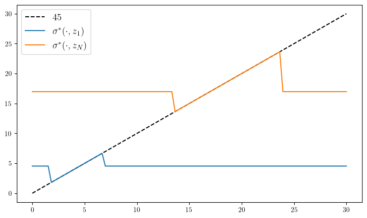
function plot_policy(; savefig=false, 
                    figname="./figures/firm_hiring_pol.pdf")
    model = create_hiring_model()
    (; β, κ, α, p, w, l_grid, z_grid, Q) = model
    σ_star = optimistic_policy_iteration(model)
    fig, ax = plt.subplots(figsize=(9, 5.2))
    ax.plot(l_grid, l_grid, "k--", label=L"45")
    ax.plot(l_grid, l_grid[σ_star[:, 1]], label=L"\sigma^*(\cdot, z_1)")
    ax.plot(l_grid, l_grid[σ_star[:, end]], label=L"\sigma^*(\cdot, z_N)")
    ax.legend(fontsize=fontsize)
end


function sim_dynamics(model, ts_length)

    (; β, κ, α, p, w, l_grid, z_grid, Q) = model
    σ_star = optimistic_policy_iteration(model)
    mc = MarkovChain(Q, z_grid)
    z_sim_idx = simulate_indices(mc, ts_length)
    z_sim = z_grid[z_sim_idx]
    l_sim_idx = Vector{Int32}(undef, ts_length)
    l_sim_idx[1] = 32
    for t in 1:(ts_length-1)
        l_sim_idx[t+1] = σ_star[l_sim_idx[t], z_sim_idx[t]]
    end
    l_sim = l_grid[l_sim_idx]

    y_sim = similar(l_sim)
    for (i, l) in enumerate(l_sim)
        y_sim[i] = p * z_sim[i] * l_sim[i]^α
    end

    t = ts_length - 1
    l_g, y_g, z_g = zeros(t), zeros(t), zeros(t)

    for i in 1:t
        l_g[i] = (l_sim[i+1] - l_sim[i]) / l_sim[i]
        y_g[i] = (y_sim[i+1] - y_sim[i]) / y_sim[i]
        z_g[i] = (z_sim[i+1] - z_sim[i]) / z_sim[i]
    end

    return l_sim, y_sim, z_sim, l_g, y_g, z_g

end



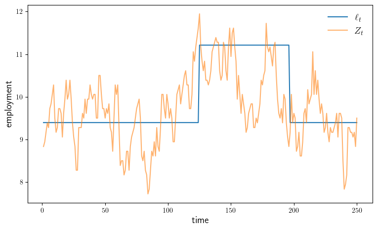
function plot_sim(; savefig=false, 
                    figname="./figures/firm_hiring_ts.pdf",
                    ts_length = 250)

    model = create_hiring_model()
    (; β, κ, α, p, w, l_grid, z_grid, Q) = model
    l_sim, y_sim, z_sim, l_g, y_g, z_g = sim_dynamics(model, ts_length)
    fig, ax = plt.subplots(figsize=(9, 5.2))
    ax.plot(1:ts_length, l_sim, label=L"\ell_t")
    ax.plot(1:ts_length, z_sim, alpha=0.6, label=L"Z_t")
    ax.legend(fontsize=fontsize, frameon=false)
    ax.set_ylabel("employment", fontsize=fontsize)
    ax.set_xlabel("time", fontsize=fontsize)

    if savefig
        fig.savefig(figname)
    end
end


function plot_growth(; savefig=false, 
                    figname="./figures/firm_hiring_g.pdf",
                    ts_length = 10_000_000)

    model = create_hiring_model()
    (; β, κ, α, p, w, l_grid, z_grid, Q) = model
    l_sim, y_sim, z_sim, l_g, y_g, z_g = sim_dynamics(model, ts_length)

    fig, ax = plt.subplots()
    ax.hist(l_g, alpha=0.6, bins=100)
    ax.set_xlabel("growth", fontsize=fontsize)

    #fig, axes = plt.subplots(2, 1)
    #series = y_g, z_g
    #for (ax, g) in zip(axes, series)
    #    ax.hist(g, alpha=0.6, bins=100)
    #    ax.set_xlabel("growth", fontsize=fontsize)
    #end

    plt.tight_layout()
    if savefig
        fig.savefig(figname)
    end
end

plot_growth (generic function with 1 method)

plot_policy()

PyObject <matplotlib.legend.Legend object at 0x7ffa29a13a90>

plot_sim(savefig=true)

plot_growth(savefig=true)

modified_opt_savings.jl

using QuantEcon, LinearAlgebra, IterTools

function create_savings_model(; β=0.98, γ=2.5,  
                                w_min=0.01, w_max=20.0, w_size=100,
                                ρ=0.9, ν=0.1, y_size=20,
                                η_min=0.75, η_max=1.25, η_size=2)
    η_grid = LinRange(η_min, η_max, η_size)  
    ϕ = ones(η_size) * (1 / η_size)  # Uniform distributoin
    w_grid = LinRange(w_min, w_max, w_size)  
    mc = tauchen(y_size, ρ, ν)
    y_grid, Q = exp.(mc.state_values), mc.p
    return (; β, γ, η_grid, ϕ, w_grid, y_grid, Q)
end



## == Functions for regular OPI == ##

"""
B(w, y, η, w′) = u(w + y - w′/η)) + β Σ v(w′, y′, η′) Q(y, y′) ϕ(η′)
"""
function B(i, j, k, l, v, model)
    (; β, γ, η_grid, ϕ, w_grid, y_grid, Q) = model
    w, y, η, w′ = w_grid[i], y_grid[j], η_grid[k], w_grid[l]
    u(c) = c^(1-γ)/(1-γ)
    c = w + y - (w′/ η)
    exp_value = 0.0
    for m in eachindex(y_grid)
        for n in eachindex(η_grid)
            exp_value += v[l, m, n] * Q[j, m] * ϕ[n]
        end
    end
    return c > 0 ? u(c) + β * exp_value : -Inf
end

"The policy operator."
function T_σ(v, σ, model)
    (; β, γ, η_grid, ϕ, w_grid, y_grid, Q) = model
    grids = w_grid, y_grid, η_grid
    w_idx, y_idx, η_idx = (eachindex(g) for g in grids)
    v_new = similar(v)
    for (i, j, k) in product(w_idx, y_idx, η_idx)
        v_new[i, j, k] = B(i, j, k, σ[i, j, k], v, model) 
    end
    return v_new
end

"Compute a v-greedy policy."
function get_greedy(v, model)
    (; β, γ, η_grid, ϕ, w_grid, y_grid, Q) = model
    w_idx, y_idx, η_idx = (eachindex(g) for g in (w_grid, y_grid, η_grid))
    σ = Array{Int32}(undef, length(w_idx), length(y_idx), length(η_idx))
    for (i, j, k) in product(w_idx, y_idx, η_idx)
        _, σ[i, j, k] = findmax(B(i, j, k, l, v, model) for l in w_idx)
    end
    return σ
end


"Optimistic policy iteration routine."
function optimistic_policy_iteration(model; tolerance=1e-5, m=100)
    (; β, γ, η_grid, ϕ, w_grid, y_grid, Q) = model
    v = zeros(length(w_grid), length(y_grid), length(η_grid))
    error = tolerance + 1
    while error > tolerance
        last_v = v
        σ = get_greedy(v, model)
        for i in 1:m
            v = T_σ(v, σ, model)
        end
        error = maximum(abs.(v - last_v))
        println("OPI current error = $error")
    end
    return get_greedy(v, model)
end


## == Functions for modified OPI == ##

"D(w, y, η, w′, g) = u(w + y - w′/η) + β g(y, w′)."
@inline function D(i, j, k, l, g, model)
    (; β, γ, η_grid, ϕ, w_grid, y_grid, Q) = model
    w, y, η, w′ = w_grid[i], y_grid[j], η_grid[k], w_grid[l]
    u(c) = c^(1-γ)/(1-γ)
    c = w + y - (w′/η)
    return c > 0 ? u(c) + β * g[j, l] : -Inf
end


"Compute a g-greedy policy."
function get_g_greedy(g, model)
    (; β, γ, η_grid, ϕ, w_grid, y_grid, Q) = model
    w_idx, y_idx, η_idx = (eachindex(g) for g in (w_grid, y_grid, η_grid))
    σ = Array{Int32}(undef, length(w_idx), length(y_idx), length(η_idx))
    for (i, j, k) in product(w_idx, y_idx, η_idx)
        _, σ[i, j, k] = findmax(D(i, j, k, l, g, model) for l in w_idx)
    end
    return σ
end


"The modified policy operator."
function R_σ(g, σ, model)
    (; β, γ, η_grid, ϕ, w_grid, y_grid, Q) = model
    w_idx, y_idx, η_idx = (eachindex(g) for g in (w_grid, y_grid, η_grid))
    g_new = similar(g)
    for (j, i′) in product(y_idx, w_idx)  # j indexes y, i′ indexes w′ 
        out = 0.0
        for j′ in y_idx                   # j′ indexes y′
            for k′ in η_idx               # k′ indexes η′
                out += D(i′, j′, k′, σ[i′, j′, k′], g, model) * 
                        Q[j, j′] * ϕ[k′]
            end
        end
        g_new[j, i′] = out
    end
    return g_new
end


"Modified optimistic policy iteration routine."
function mod_opi(model; tolerance=1e-5, m=100)
    (; β, γ, η_grid, ϕ, w_grid, y_grid, Q) = model
    g = zeros(length(y_grid), length(w_grid))
    error = tolerance + 1
    while error > tolerance
        last_g = g
        σ = get_g_greedy(g, model)
        for i in 1:m
            g = R_σ(g, σ, model)
        end
        error = maximum(abs.(g - last_g))
        println("OPI current error = $error")
    end
    return get_g_greedy(g, model)
end


# == Simulations and inequality measures == #

function simulate_wealth(m)

    model = create_savings_model()
    (; β, γ, η_grid, ϕ, w_grid, y_grid, Q) = model
    σ_star = mod_opi(model)

    # Simulate labor income
    mc = MarkovChain(Q)
    y_idx_series = simulate(mc, m)

    # IID Markov chain with uniform draws
    l = length(η_grid)
    mc = MarkovChain(ones(l, l) * (1/l))
    η_idx_series = simulate(mc, m)

    w_idx_series = similar(y_idx_series)
    w_idx_series[1] = 1
    for t in 1:(m-1)
        i, j, k = w_idx_series[t], y_idx_series[t], η_idx_series[t]
        w_idx_series[t+1] = σ_star[i, j, k]
    end

    w_series = w_grid[w_idx_series]
    return w_series
end


function lorenz(v)  # assumed sorted vector
    S = cumsum(v)  # cumulative sums: [v[1], v[1] + v[2], ... ]
    F = (1:length(v)) / length(v)
    L = S ./ S[end]
    return (; F, L) # returns named tuple
end


gini(v) = (2 * sum(i * y for (i,y) in enumerate(v))/sum(v)
           - (length(v) + 1))/length(v)


# == Plots == #

using PyPlot
using LaTeXStrings
PyPlot.matplotlib[:rc]("text", usetex=true) # allow tex rendering
fontsize=16



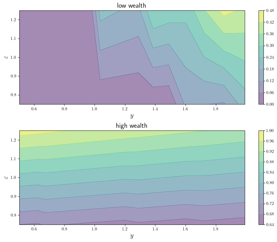
function plot_contours(; savefig=false, 
                         figname="./figures/modified_opt_savings_1.pdf")

    model = create_savings_model()
    (; β, γ, η_grid, ϕ, w_grid, y_grid, Q) = model
    σ_star = optimistic_policy_iteration(model)

    fig, axes = plt.subplots(2, 1, figsize=(10, 8))
    y_idx, η_idx = eachindex(y_grid), eachindex(η_grid)
    H = zeros(length(y_grid), length(η_grid))

    w_indices = (1, length(w_grid))
    titles = "low wealth", "high wealth"
    for (ax, w_idx, title) in zip(axes, w_indices, titles)

        for (i_y, i_ϵ) in product(y_idx, η_idx)
            w, y, η = w_grid[w_idx], y_grid[i_y], η_grid[i_ϵ]
            H[i_y, i_ϵ] = w_grid[σ_star[w_idx, i_y, i_ϵ]] / (w+y)
        end

        cs1 = ax.contourf(y_grid, η_grid, transpose(H), alpha=0.5)
        plt.colorbar(cs1, ax=ax) #, format="%.6f")

        ax.set_title(title, fontsize=fontsize)
        ax.set_xlabel(L"y", fontsize=fontsize)
        ax.set_ylabel(L"\varepsilon", fontsize=fontsize)
    end

    plt.tight_layout()
    if savefig
        fig.savefig(figname)
    end
end


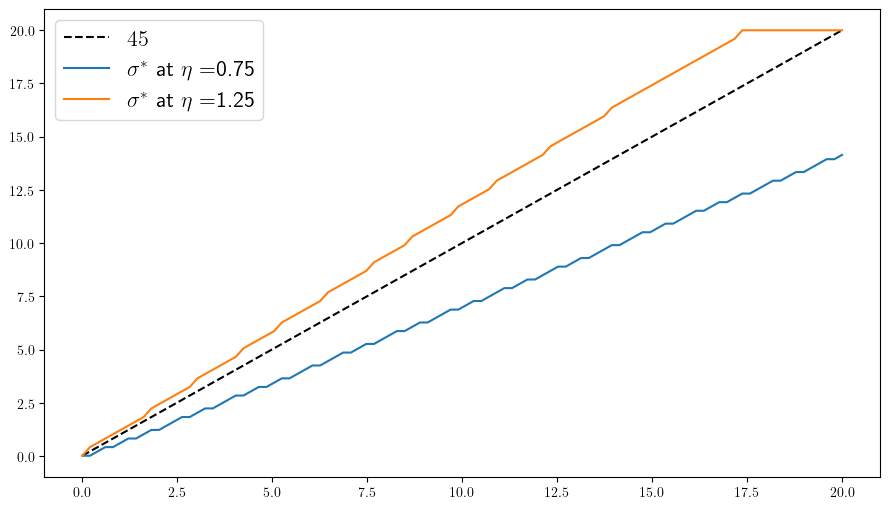
function plot_policies(; savefig=false, 
                         figname="./figures/modified_opt_savings_2.pdf")

    model = create_savings_model()
    (; β, γ, η_grid, ϕ, w_grid, y_grid, Q) = model
    σ_star = mod_opi(model)
    y_bar = floor(Int, length(y_grid) / 2)  # Index of mid-point of y_grid

    fig, ax = plt.subplots(figsize=(9, 5.2))
    ax.plot(w_grid, w_grid, "k--", label=L"45")

    for (i, η) in enumerate(η_grid)
        label = L"\sigma^*" * " at " * L"\eta = " * "$η"
        ax.plot(w_grid, w_grid[σ_star[:, y_bar, i]], label=label)
    end
    ax.legend(fontsize=fontsize)

    plt.tight_layout()
    if savefig
        fig.savefig(figname)
    end
end


function plot_time_series(; m=2_000,
                           savefig=false, 
                           figname="./figures/modified_opt_savings_ts.pdf")

    w_series = simulate_wealth(m)
    fig, ax = plt.subplots(figsize=(9, 5.2))
    ax.plot(w_series, label=L"w_t")
    ax.legend(fontsize=fontsize)
    ax.set_xlabel("time", fontsize=fontsize)
    if savefig
        fig.savefig(figname)
    end

end

function plot_histogram(; m=1_000_000,
                           savefig=false, 
                           figname="./figures/modified_opt_savings_hist.pdf")

    w_series = simulate_wealth(m)
    g = round(gini(sort(w_series)), digits=2)
    fig, ax = plt.subplots(figsize=(9, 5.2))
    ax.hist(w_series, bins=40, density=true)
    ax.set_xlabel("wealth", fontsize=fontsize)
    ax.text(15, 0.7, "Gini = $g", fontsize=fontsize)
    if savefig
        fig.savefig(figname)
    end

end


function plot_lorenz(; m=1_000_000,
                           savefig=false, 
                           figname="./figures/modified_opt_savings_lorenz.pdf")

    w_series = simulate_wealth(m)
    (; F, L) = lorenz(sort(w_series))

    fig, ax = plt.subplots(figsize=(9, 5.2))
    ax.plot(F, F, label="Lorenz curve, equality")
    ax.plot(F, L, label="Lorenz curve, wealth distribution")
    ax.legend()
    if savefig
        fig.savefig(figname)
    end

end

plot_lorenz (generic function with 1 method)

plot_contours(savefig=true)

OPI current error = 38.399920491529734

OPI current error = 4.066951180848044

OPI current error = 4.6380954261438845

OPI current error = 1.3260813588221083

OPI current error = 0.38722029225052523

OPI current error = 0.09428546775951219

OPI current error = 0.02026455329022525

OPI current error = 0.002633073607984926

OPI current error = 0.00013614255682270482

OPI current error = 7.911990667963664e-6

plot_policies(savefig=true)

OPI current error = 37.35040200118496

OPI current error = 4.066625094726078

OPI current error = 3.892585870289693

OPI current error = 1.1681955052615045

OPI current error = 0.3343174765677297

OPI current error = 0.06611271436991473

OPI current error = 0.010680300539267051

OPI current error = 0.0009714030350238545

OPI current error = 7.058042499252792e-5

OPI current error = 7.91199024874345e-6

plot_time_series(savefig=true)

OPI current error = 37.35040200118496

OPI current error = 4.066625094726078

OPI current error = 3.892585870289693

OPI current error = 1.1681955052615045

OPI current error = 0.3343174765677297

OPI current error = 0.06611271436991473

OPI current error = 0.010680300539267051

OPI current error = 0.0009714030350238545

OPI current error = 7.058042499252792e-5

OPI current error = 7.91199024874345e-6

plot_histogram(savefig=true)

OPI current error = 37.35040200118496

OPI current error = 4.066625094726078

OPI current error = 3.892585870289693

OPI current error = 1.1681955052615045

OPI current error = 0.3343174765677297

OPI current error = 0.06611271436991473

OPI current error = 0.010680300539267051

OPI current error = 0.0009714030350238545

OPI current error = 7.058042499252792e-5

OPI current error = 7.91199024874345e-6

plot_lorenz(savefig=true)

OPI current error = 37.35040200118496

OPI current error = 4.066625094726078

OPI current error = 3.892585870289693

OPI current error = 1.1681955052615045

OPI current error = 0.3343174765677297

OPI current error = 0.06611271436991473

OPI current error = 0.010680300539267051

OPI current error = 0.0009714030350238545

OPI current error = 7.058042499252792e-5

OPI current error = 7.91199024874345e-6