Chapter 4: Optimal Stopping#
firm_exit.py#
"""
Firm valuation with exit option.
"""
from quantecon.markov import tauchen
from quantecon import compute_fixed_point
import numpy as np
from collections import namedtuple
from numba import njit
# NamedTuple Model
Model = namedtuple("Model", ("n", "z_vals", "Q", "β", "s"))
def create_exit_model(
n=200, # productivity grid size
ρ=0.95, μ=0.1, ν=0.1, # persistence, mean and volatility
β=0.98, s=100.0 # discount factor and scrap value
):
"""
Creates an instance of the firm exit model.
"""
mc = tauchen(n, ρ, ν, mu=μ)
z_vals, Q = mc.state_values, mc.P
return Model(n=n, z_vals=z_vals, Q=Q, β=β, s=s)
@njit
def no_exit_value(model):
"""Compute value of firm without exit option."""
n, z_vals, Q, β, s = model
I = np.identity(n)
return np.linalg.solve((I - β * Q), z_vals)
@njit
def T(v, model):
"""The Bellman operator Tv = max{s, π + β Q v}."""
n, z_vals, Q, β, s = model
h = z_vals + β * np.dot(Q, v)
return np.maximum(s, h)
@njit
def get_greedy(v, model):
"""Get a v-greedy policy."""
n, z_vals, Q, β, s = model
σ = s >= z_vals + β * np.dot(Q, v)
return σ
def vfi(model):
"""Solve by VFI."""
v_init = no_exit_value(model)
v_star = compute_fixed_point(lambda v: T(v, model), v_init, error_tol=1e-6,
max_iter=1000, print_skip=25)
σ_star = get_greedy(v_star, model)
return v_star, σ_star
# Plots
import matplotlib.pyplot as plt
import matplotlib.pyplot as plt
plt.rcParams.update({"text.usetex": True, "font.size": 14})
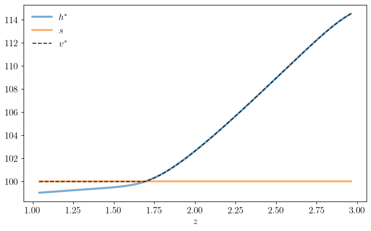
def plot_val(savefig=False,
figname="./figures/firm_exit_1.pdf"):
fig, ax = plt.subplots(figsize=(9, 5.2))
model = create_exit_model()
n, z_vals, Q, β, s = model
v_star, σ_star = vfi(model)
h = z_vals + β * np.dot(Q, v_star)
ax.plot(z_vals, h, "-", linewidth=3, alpha=0.6, label=r"$h^*$")
ax.plot(z_vals, s * np.ones(n), "-", linewidth=3, alpha=0.6, label=r"$s$")
ax.plot(z_vals, v_star, "k--", linewidth=1.5, alpha=0.8, label=r"$v^*$")
ax.legend(frameon=False)
ax.set_xlabel(r"$z$")
if savefig:
fig.savefig(figname)
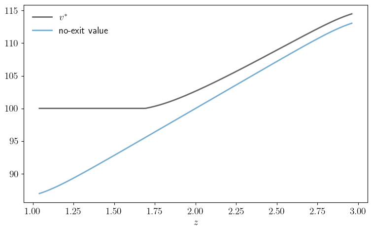
def plot_comparison(savefig=False,
figname="./figures/firm_exit_2.pdf"):
fig, ax = plt.subplots(figsize=(9, 5.2))
model = create_exit_model()
n, z_vals, Q, β, s = model
v_star, σ_star = vfi(model)
w = no_exit_value(model)
ax.plot(z_vals, v_star, "k-", linewidth=2, alpha=0.6, label="$v^*$")
ax.plot(z_vals, w, linewidth=2, alpha=0.6, label="no-exit value")
ax.legend(frameon=False)
ax.set_xlabel(r"$z$")
if savefig:
fig.savefig(figname)
plot_val()
Iteration    Distance       Elapsed (seconds)
---------------------------------------------
25           3.581e-02      8.320e-01
50           1.723e-02      8.329e-01
75           6.768e-03      8.335e-01
100          2.643e-03      8.341e-01
125          1.043e-03      8.347e-01
150          4.139e-04      8.353e-01
175          1.643e-04      8.359e-01
200          6.522e-05      8.366e-01
225          2.589e-05      8.372e-01
250          1.028e-05      8.379e-01
275          4.080e-06      8.385e-01
300          1.619e-06      8.391e-01
314          9.653e-07      8.395e-01
Converged in 314 steps
plot_comparison()
Iteration    Distance       Elapsed (seconds)
---------------------------------------------
25           3.581e-02      7.725e-04
50           1.723e-02      1.290e-03
75           6.768e-03      1.779e-03
100          2.643e-03      2.271e-03
125          1.043e-03      2.758e-03
150          4.139e-04      3.296e-03
175          1.643e-04      3.823e-03
200          6.522e-05      4.346e-03
225          2.589e-05      4.831e-03
250          1.028e-05      5.316e-03
275          4.080e-06      5.803e-03
300          1.619e-06      6.342e-03
314          9.653e-07      6.663e-03
Converged in 314 steps
american_option.py#
"""
Valuation for finite-horizon American call options in discrete time.
"""
from quantecon.markov import tauchen, MarkovChain
from quantecon import compute_fixed_point
import numpy as np
from collections import namedtuple
from numba import njit, prange
# NamedTuple Model
Model = namedtuple("Model", ("t_vals", "z_vals","w_vals", "Q",
"φ", "T", "β", "K"))
@njit
def exit_reward(t, i_w, i_z, T, K):
"""Payoff to exercising the option at time t."""
return (t < T) * (i_z + i_w - K)
def create_american_option_model(
n=100, μ=10.0, # Markov state grid size and mean value
ρ=0.98, ν=0.2, # persistence and volatility for Markov state
s=0.3, # volatility parameter for W_t
r=0.01, # interest rate
K=10.0, T=200): # strike price and expiration date
"""
Creates an instance of the option model with log S_t = Z_t + W_t.
"""
t_vals = np.arange(T+1)
mc = tauchen(n, ρ, ν)
z_vals, Q = mc.state_values + μ, mc.P
w_vals, φ, β = np.array([-s, s]), np.array([0.5, 0.5]), 1 / (1 + r)
return Model(t_vals=t_vals, z_vals=z_vals, w_vals=w_vals, Q=Q,
φ=φ, T=T, β=β, K=K)
@njit(parallel=True)
def C(h, model):
"""The continuation value operator."""
t_vals, z_vals, w_vals, Q, φ, T, β, K = model
Ch = np.empty_like(h)
z_idx, w_idx = np.arange(len(z_vals)), np.arange(len(w_vals))
for i in prange(len(t_vals)):
t = t_vals[i]
for i_z in prange(len(z_vals)):
out = 0.0
for i_w_1 in prange(len(w_vals)):
for i_z_1 in prange(len(z_vals)):
t_1 = min(t + 1, T)
out += max(exit_reward(t_1, w_vals[i_w_1], z_vals[i_z_1], T, K),
h[t_1, i_z_1]) * Q[i_z, i_z_1] * φ[i_w_1]
Ch[t, i_z] = β * out
return Ch
def compute_cvf(model):
"""
Compute the continuation value function by successive approx.
"""
h_init = np.zeros((len(model.t_vals), len(model.z_vals)))
h_star = compute_fixed_point(lambda h: C(h, model), h_init,
error_tol=1e-6, max_iter=1000,
print_skip=25)
return h_star
# Plots
import matplotlib.pyplot as plt
import matplotlib.pyplot as plt
plt.rcParams.update({"text.usetex": True, "font.size": 14})
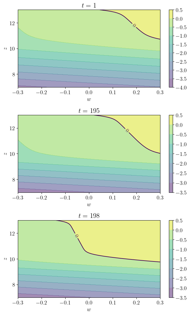
def plot_contours(savefig=False,
figname="./figures/american_option_1.pdf"):
model = create_american_option_model()
t_vals, z_vals, w_vals, Q, φ, T, β, K = model
h_star = compute_cvf(model)
fig, axes = plt.subplots(3, 1, figsize=(7, 11))
z_idx, w_idx = np.arange(len(z_vals)), np.arange(len(w_vals))
H = np.zeros((len(w_vals), len(z_vals)))
for (ax_index, t) in zip(range(3), (1, 195, 198)):
ax = axes[ax_index]
for i_w in prange(len(w_vals)):
for i_z in prange(len(z_vals)):
H[i_w, i_z] = exit_reward(t, w_vals[i_w], z_vals[i_z], T,
K) - h_star[t, i_z]
cs1 = ax.contourf(w_vals, z_vals, np.transpose(H), alpha=0.5)
ctr1 = ax.contour(w_vals, z_vals, np.transpose(H), levels=[0.0])
plt.clabel(ctr1, inline=1, fontsize=13)
plt.colorbar(cs1, ax=ax)
ax.set_title(f"$t={t}$")
ax.set_xlabel(r"$w$")
ax.set_ylabel(r"$z$")
fig.tight_layout()
if savefig:
fig.savefig(figname)
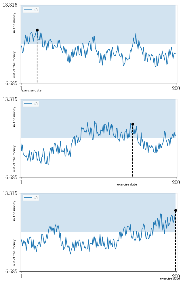
def plot_strike(savefig=False,
fontsize=9,
figname="./figures/american_option_2.pdf"):
model = create_american_option_model()
t_vals, z_vals, w_vals, Q, φ, T, β, K = model
h_star = compute_cvf(model)
# Built Markov chains for simulation
z_mc = MarkovChain(Q, z_vals)
P_φ = np.zeros((len(w_vals), len(w_vals)))
for i in range(len(w_vals)): # Build IID chain
P_φ[i, :] = φ
w_mc = MarkovChain(P_φ, w_vals)
y_min = np.min(z_vals) + np.min(w_vals)
y_max = np.max(z_vals) + np.max(w_vals)
fig, axes = plt.subplots(3, 1, figsize=(7, 12))
for ax in axes:
# Generate price series
z_draws = z_mc.simulate_indices(T, init=int(len(z_vals) / 2 - 10))
w_draws = w_mc.simulate_indices(T)
s_vals = z_vals[z_draws] + w_vals[w_draws]
# Find the exercise date, if any.
exercise_date = T + 1
for t in range(T):
k = exit_reward(t, w_vals[w_draws[t]], z_vals[z_draws[t]], T, K) - \
h_star[w_draws[t], z_draws[t]]
if k >= 0:
exercise_date = t
if exercise_date >= T:
print("Warning: Option not exercised.")
else:
# Plot
ax.set_ylim(y_min, y_max)
ax.set_xlim(0, T+1)
ax.fill_between(range(T), np.ones(T) * K, np.ones(T) * y_max, alpha=0.2)
ax.plot(range(T), s_vals, label=r"$S_t$")
ax.plot((exercise_date,), (s_vals[exercise_date]), "ko")
ax.vlines((exercise_date,), 0, (s_vals[exercise_date]), ls="--", colors="black")
ax.legend(loc="upper left", fontsize=fontsize)
ax.text(-10, 11, "in the money", fontsize=fontsize, rotation=90)
ax.text(-10, 7.2, "out of the money", fontsize=fontsize, rotation=90)
ax.text(exercise_date-20, 6,
"exercise date", fontsize=fontsize)
ax.set_xticks((1, T))
ax.set_yticks((y_min, y_max))
if savefig:
fig.savefig(figname)
plot_contours()
Iteration    Distance       Elapsed (seconds)
---------------------------------------------
25           6.682e-03      1.712e+00
50           3.997e-03      1.793e+00
75           2.923e-03      1.875e+00
100          1.960e-03      1.961e+00
125          1.242e-03      2.043e+00
150          7.739e-04      2.124e+00
175          4.811e-04      2.207e+00
200          0.000e+00      2.289e+00
Converged in 200 steps
plot_strike()
Iteration    Distance       Elapsed (seconds)
---------------------------------------------
25           6.682e-03      8.388e-02
50           3.997e-03      1.649e-01
75           2.923e-03      2.513e-01
100          1.960e-03      3.349e-01
125          1.242e-03      4.179e-01
150          7.739e-04      5.030e-01
175          4.811e-04      5.860e-01
200          0.000e+00      6.693e-01
Converged in 200 steps