This section provides a brief review of basic analysis and linear algebra. The material contained here should be covered in intermediate mathematical economics courses or, if not, in math boot camp at the very start of a graduate program.
(For those who want a slower treatment of the analysis section, we recommend Bartle & Sherbert (2011), which is carefully constructed and beautifully written. High quality texts on linear algebra at the right level for this course include Jänich (1994), Meyer (2000), Aggarwal (2020) and Cohen (2021).)
A set is an arbitrary collection of objects. Individual objects are called elements of the set. We assume the reader is familiar with basic set operations such as intersections and unions. If A is a finite set, then ∣A∣ is the number of elements in A. Powers applied to sets indicate Cartesian products, so that
A2:=A×A:={(a,a′):a∈A,a′∈A},etc.
Throughout, ℘(A) is the power set of A, consisting of all subsets of A. For example,
A={1,2}⟹℘(A)={∅,{1},{2},A}.
Let N be the natural numbers, Z be the integers, Q be the rational numbers and R be the reals (i.e., the union of the rational and irrational numbers). For x,y in R, we let
Let S be any set. A relation∼ on S is a nonempty subset of S×S. It is customary to write x∼y rather than (x,y)∈∼ to indicate that (x,y) is in ∼. A relation ∼ on S is called an equivalence relation if, for all x,y,z∈S, we have
(reflexivity) x∼x,
(symmetry) x∼y implies y∼x and
(transitivity) x∼y and y∼z implies x∼z.
Any equivalence relation on S induces a partition of S into a collection of mutually disjoint subsets such that their union exhausts S. These subsets are called equivalence classes. They can be constructed by taking, for each x∈S, the set of all elements that are equivalent to x.
A functionf from set A to set B is a rule, written f:A→B or a↦f(a), that associates each element a of A with one and only one element f(a) of B. The set A is called the domain of f and B is called the codomain. The range or image of f is
range(f):={b∈B:b=f(a) for some a∈A}.
A function f:A→B is called
one-to-one if f(a)=f(a′) implies a=a′,
onto if range(f)=B, and
a bijection or one-to-one correspondence if f is both onto and one-to-one.
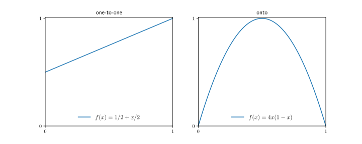
The left panel of Figure 6.1 shows a one-to-one function on (0,1). This function is not onto, however. For example, there exists no x∈(0,1) with f(x)=1/4. The right panel of Figure 6.1 shows an onto function, with range(f)=(0,1). This function is not one-to-one, however. For example, f(1/4)=f(3/4)=3/4.
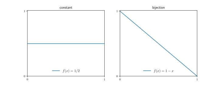
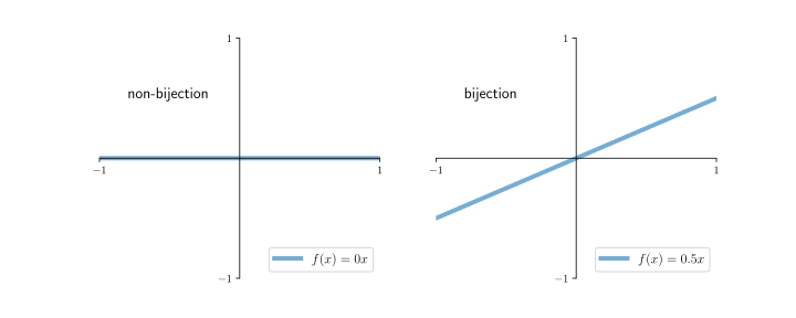
The left panel of Figure 6.2 gives an example of a function which is neither one-to-one nor onto. The right panel of Figure 6.2 gives an example of a bijection.
Figure 6.2:Some functions are bijections and some are not
One motivation for our interest in the basic properties of functions is that we wish to solve inverse problems. For an arbitrary nonempty set S and a function f:S→S, an abstraction of an inverse problem is solving y=f(x) for x∈S.
Prior to stating the next result, we recall that an inverse function for f:S→S is a function g:S→S such that f∘g=g∘f=I, where I is the identity map on S. The inverse function of f is often written as f−1.
Here is a nice logical exercise that turns out to be useful when we solve linear inverse problems.
If S is any set and f:S→R, we call f a real-valued function. The set of all real-valued functions on S is denoted RS. When S has n elements, RS is the same set as Rn expressed in different notation. The next lemma clarifies.
The lemma just states that a function h can be identified by the set of values that it takes on S, which is an n-tuple of real numbers. We use this identification routinely in what follows.
The indicator function of logical statement P is denoted 1{P} and takes value 1 (resp., 0) if P is true (resp., false).
If A⊂S, where S is any set, then 1A(x):=1{x∈A} for all x∈S.
A nonempty set S is called countable if it is finite or can be placed in one-to-one correspondence with the natural numbers N. In the second case we can enumerate S by writing it as {x1,x2,…}. Any nonempty set S that fails to be countable is called uncountable. For example, Z and Q are countable, whereas R and every nontrivial interval in R are uncountable.
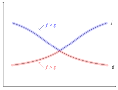
In general, if f and g are real-valued functions defined on some common set S and α is a scalar, then f+g, αf, fg, etc., are functions on S defined by
Let S be any set. A self-map on S is a function G from S to itself. When working with self-maps in arbitrary sets it is common to write the image of x under G as Gx rather than G(x). We often follow this convention.
Given a self-map G on S, a point x∈S is called a fixed point of G if Gx=x.
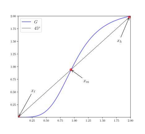
Figure 6.4 shows another example, for a self-map G on S=[0,2]. Fixed points are numbers x∈[0,2] where G meets the 45 degree line. In this case there are three.
One of the most common techniques for solving systems of nonlinear equations in applied mathematics—and quantitative economics—is to convert them into fixed point problems and then apply fixed point theory. We will see many applications of this technique.
Figure 6.4:Graph and fixed points of G:x↦2.125/(1+x−4)
An n-vector x is a tuple of n numbers x=(x1,…,xn) where xi∈R for each i∈[n]. In general, x is neither a row vector nor a column vector—which coincides with the perspective of most scientific computing environments, where the basic vector structure is a flat array. When using matrix algebra, vectors are treated as column vectors unless otherwise stated.
The two most fundamental vector operations are vector addition and scalar multiplication. These operations act pointwise, so that, when α∈R and x,y∈Rn,
We recall some elementary facts about C, the set of complex numbers.
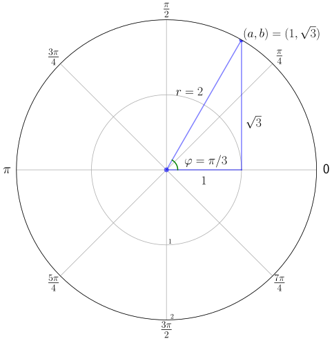
Each element of C can be understood as a point (a,b)∈R2. In fact C is just R2 endowed with a special form of multiplication. The point (a,b) is more often written as a+ib. We elaborate below.
The first and second projections of (a,b) are written as Re(a,b)=a and Im(a,b)=b and called the real and nonreal (or imaginary) part respectively. The symbol i represents the point (0,1)∈C. As is traditional, in the context of complex numbers, the complex number (a,0)∈C is often written more simply as a. With addition and scalar multiplication defined pointwise, this means that, as expected,
(a,b)=(a,0)+(0,b)=(a,0)+(0,1)b=a+ib.
Let z=(a,b). The modulus of z is written ∣z∣ and defined as the Euclidean norm (a2+b2)1/2 of the tuple (a,b). The two-dimensional Euclidean space is then endowed with a new operation called multiplication, which is defined by
Note that, under this rule and our conventions, i2=(0,1)(0,1)=(−1,0)=−1.
As in the real case, the exponential ez is defined for z∈C by ∑k⩾0zk/(k!). It can be shown that, under this extension, the exponential function continues to enjoy the additive property ez1+z2=ez1ez2. As a result, ea+ib=eaeib.
Rather than providing its coordinates, another way to represent a vector z=(a,b)∈R2, and hence in C, is by providing a pair (r,φ) where r>0 is understood as the length of the vector and φ∈[0,2π) is the angle. This translates to Euclidean coordinates via
In this text, operations on real numbers such as ∣⋅∣ and ∨ are applied to vectors pointwise. For example, for vectors a=(ai) and b=(bi) in Rd, we set
A small amount of thought will convince you that, with this convention plus the pointwise order over vectors, the order-theoretic inequalities and identities listed in Section 6.1.1.1 also hold for vectors in Rd. (For example, ∣a+b∣⩽∣a∣+∣b∣ for any a,b,c∈Rd.)
If P=Q=R and ⪯ and ⊴ are both equal to ⩽, the standard order on R, then the order-preserving property reduces to the usual notion of an increasing function (i.e., nondecreasing function), and we will use the terms “increasing” and “order-preserving” interchangeably in this setting.[2]
In addition, if S=g maps A⊂R into R, then we will call g
Let’s now recall the basics of convergence and continuity.
Given any set S, an S-valued sequence(xn):=(xn)n∈N is a function n↦xn from N to S. If S=R, we call (xn) a real-valued sequence. A subsequence of (xn)n∈N is a sequence of the form (xσ(n))n∈N where σ is a strictly increasing function from N to itself. You can think of forming a subsequence from a sequence by deleting some of its elements—while still retaining infinitely many.
In computer science and statistics, it is common to classify sequences according to their asymptotic behavior. Often this is done via big O notation, where, for a real-valued sequence (xn), we write (xn)=O(gn) if there exists a nonnegative sequence (gn) and a constant M<∞ such that ∣xn∣⩽Mgn for all n∈N.
The following definition is fundamental to what follows: a real-valued sequence (xn)converges to x∈R and write xn→x if
for each ε>0, there is an N∈N such that ∣xn−x∣<ε whenever n⩾N.
Let’s state some elementary limit laws that are used without comment throughout. (You can review the proofs in sources such as Bartle & Sherbert (2011)).
A sequence (xn) is called bounded if there is an M∈R such that ∣xn∣⩽M for all n∈N. It is called
monotone increasing if xn⩽xn+1 for all n∈N, and
monotone decreasing if xn⩾xn+1 for all n.
The sequence is called monotone if it is either monotone increasing or decreasing. The next theorem, concerning monotone sequences, is a deep result about the structure of R.
The intuitive meaning of the “if” part of Theorem 6.1.3 is that monotone bounded sequences always converge to some point in R because R contains no gaps. This statement is closely related to the “completeness” property of the real line, which is discussed in Bartle & Sherbert (2011) and many other texts on real analysis.
Next let’s consider series. Given a sequence (xn) in R, we set
n⩾1∑xn:=N→∞limn=1∑Nxn whenever the limit exists in R.
More generally, given arbitrary countable S and g∈RS, we write ∑x∈Sg(x)=M if there exists an enumeration (xn)n∈N of S such that ∑n⩾1∣g(xn)∣ is finite and, in addition, ∑n⩾1g(xn)=M.[3]
Now we review the metric properties of Rd, for some d∈N, when distance between vectors x,y∈Rd is understood in terms of Euclidean norm deviation ∥x−y∥. The notion of convergence for real-valued sequences extends naturally to this setting: sequence (xn) in Rd is said to converge to x∈Rd if
for each ε>0, there is an N∈N such that ∥xn−x∥<ε whenever n⩾N.
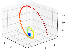
In this case we write xn→x. Figure 6.6 shows a sequence converging to the origin in R3, with colder colors being later in the sequence.
Figure 6.6:Convergence of a sequence to the origin in R3
Given any point u∈Rd and ε>0, the ε-ball around u is the set
Bε(u):={v∈Rd:∥u−v∥<ε}.
With this terminology, we can say that (xn) converges to x∈Rd if the sequence (xn) is eventually in any ε-ball around x.
A sequence (xn)⊂Rd is called Cauchy if, for all ε>0, there exists an N∈N with ∣xn−xm∣<ε whenever n,m⩾N.
It is a fundamental result of analysis, stemming from axiomatic properties of the reals, that the converse is also true:
A point u∈A⊂Rd is called interior to A if there exists an ε>0 such that Bε(u)⊂A.
A subset G of Rd is called open in Rd if every u∈G is interior to G. A subset F of Rd is called closed if, given any sequence (xn) satisfying xn∈F for all n∈N and xn→x for some x∈Rd, the point x is in F. In other words, F contains the limit points of all convergent sequences that take values in F.
A subset B of Rd is called bounded if there exists a finite M such that ∥b∥⩽M for all b∈B. A subset K of Rd is called compact in Rd if every sequence in K has a subsequence converging to some point in K. The Bolzano–Weierstrass theorem tells us that K is compact if and only if K is closed and bounded.
If A⊂Rd, then f:A→Rk is called continuous at x∈A if, for each sequence (xn)⊂A with xn→x, we have f(xn)→f(x) in Rk. If f is continuous at all x∈A then we call fcontinuous on A.
More generally, every polynomial function is continuous on R. The elementary functions sin, cos, exp and log are all continuous on their domains.
The next lemma is helpful in locating fixed points.
A subset E of Rn is called a linear subspace of Rn if
x,y∈E and α,β∈R⟹αx+βy∈E.
In other words, E is closed under the operations of addition and scalar multiplication; that is, (i) α∈R and x∈E implies αx∈E and (ii) x,y∈E implies x+y∈E.
A linear combination of vectors v1,…,vk in Rn is a vector of the form
α1v1+⋯+αkvk where (α1,…,αk)∈Rk.
The set of all linear combinations of elements of F⊂Rn is called the span of F and written as spanF.
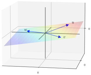
Figure 6.7 shows the linear subspace spanned by the three vectors
The subspace H in which these vectors lie is, in fact, the set of all x∈R3 such that ⟨x,c⟩=0, with c=(−0.2,−0.1,1). This plane is a two-dimensional object. While we make this terminology precise in Section 6.1.4.2, the key idea is that
at least two vectors are required to span H and
any additional vectors will not increase the span.
On the other hand, we cannot omit an element of the basis {δ1,…,δn} and still span Rn. The next theorem generalizes this idea.
See, for example, Jänich (1994). Theorem 6.1.7 captures the notion that linear independence of a set of vectors means linear diversity, which allows the span to be large.
Let V be a linear subspace of Rn. A set B⊂V is called a basis for V if B is linearly independent and spanB=V.
The key idea behind a basis is this: If S={v1,…,vk} spans some linear subspace V, then each element of V can be written as a linear combination of elements of S. If S is, in addition, linearly independent (and hence a basis), then this representation is unique: for each u∈V, there is exactly one (α1,…,αk)∈Rk such that
u=α1v1+⋯+αkvk.
Indeed, if u=β1v1+⋯+βkvk is another representation, then, subtracting this equality from the last, we have
(α1−β1)v1+⋯+(αk−βk)vk=0.
Because S is assumed to be linearly independent, this yields αi=βi for all i∈[k].
Not surprisingly, given their name, the canonical basis vectors E:={δ1,…,δn} serve as a basis for the whole space Rn. The representation (6.11), with coefficients αi=⟨x,δi⟩, is unique.
Theorem 6.1.8 is a relatively deep result. See, for example, Jänich (1994). The common number of bases in (ii) is called the dimension of V and written as dimV.
The “nonzero” qualification in Theorem 6.1.8 is included for the case V={0}, which is a linear subspace that lacks any basis. It is sensible, and standard, to agree that the linear subspace {0}⊂Rn has dimension zero.
Dimensionality is one measure of the “size” of a linear subspace. To illustrate, consider the system Ax=b where A∈Mn×k, x∈Rk and b∈Rn. Is there an x that solves this system? This will be more likely if the column space of A is large (see Example 6.1.13). A large span will be obtained when the columns are linearly “diverse.” In other words, our hope is that there exists a large subset of the columns of A that is linearly independent, which in turn will be true when the span of A is high-dimensional.
To quantify these ideas, we define the rank of A as
rankA:=dim(rangeA)= dimension of the column space of A.
See, for example, Chapter 2 of Aggarwal (2020) or Chapter 5 of Jänich (1994). In view of Exercise 6.1.26, for A∈Mn×k, we have rankA⩽k. If rankA=k, then A is said to have full column rank.
In general, a linear subspace V contains within itself many other linear subspaces. (For example, a plane passing through the origin contains many lines that pass through the origin, each one of which is a linear subspace.) However, there is no proper subspace of V (i.e., no linear subspace contained in and distinct from V) with the same dimension as V. The next theorem records this fact.
Part (ii) is related to Figure 6.7. The plane in that figure is 2-dimensional, as we confirm in Section 6.1.4.3 below. Any three vectors lying in the plane are linearly dependent.
We will see in the following chapters that many nonlinear dynamic models and estimation problems can be expressed in terms of linear operations in high-dimensional spaces. We now state the definition of linear maps and their connection to matrices.
A function u↦Au from Rk to Rn is called linear if
A(αu+βv)=αAu+βAv for all α,β∈R and all u,v in Rk.
In this context, A is sometimes called an operator rather than a function, but the meaning is the same.
One of the most striking and useful properties of linear operators is that the one-to-one property and the onto property are equivalent when the domain and codomain agree:
The proof can be found in Jänich (1994) or Stachurski (2016). Figure 6.8 illustrates in the one-dimensional case. The linear map f(x)=αx is onto if and only if it is one-to-one, which occurs if and only if α=0.
Figure 6.8:Equivalence of the onto and one-to-one properties
A matrix A∈Mn×k is a linear function from Rk to Rn when identified with the mapping that sends a (column) vector u in Rk into the vector Au in Rn. In fact it is fundamental that, for every linear map A:Rk→Rn, there exists a unique MA∈Mn×k such that
(see, e.g., Kreyszig (1978), §2.9). Thus, the set of linear maps and the set of matrices are in one-to-one correspondence in the finite dimensional setting.
In Exercise 6.1.21, you confirmed that, for a given nonzero c∈Rn, the subset of Rn defined by H:={x∈Rn:⟨c,x⟩=0} is a linear subspace of Rn. Any set H of this form is called a linear hyperplane in Rn. The vector c is called the normal vector of the hyperplane.
In the discussion after Figure 6.7, we claimed that the linear hyperplane has shown there is a two-dimensional subset of R3. The next example generalizes this idea.
A crucial task in applied modeling is solving linear systems such as Ax=b, where A is a matrix and x and b are conformable column vectors. The system can be underdetermined, overdetermined or exactly determined (i.e., same number of equations as unknowns). In this section we consider the last case, where the theory is straightforward.
Let A and B be in Mn×n and suppose that AB=BA=I. Then B is called the inverse of A, written as A−1, while A is said to be invertible or nonsingular.
The next theorem states that, for square matrices, the property of having either a left or a right inverse is equivalent to nonsingularity.
Consider the linear system Ax=b, where A∈Mn×n and b∈Rn. We seek a solution x∈Rn. The next theorem provides conditions under which such an x is always uniquely identified.
The symbol detA represents the determinant of A. For the definition, see, for example, Jänich (1994) or Cohen (2021). We note only that, for n×n matrices A and B,
det(AB)=det(A)det(B),
det(αA)=αndetA for all α∈R, and
det(A−1)=(detA)−1 whenever A is nonsingular.
Most of the equivalences in Theorem 6.1.14 can be established from the results presented above. The key idea is that, under these equivalent conditions, the columns of A form a basis of Rn, and hence any b∈Rn can be expressed uniquely as a linear combination of elements of these columns. In other words, there exists a unique x∈Rn with Ax=b. The remaining points are just equivalent ways of saying that the columns of A form a basis of Rn.
We recall that vectors u,v in Rn are called orthogonal and we write u⊥v if ⟨u,v⟩=0. For a linear subspace L of Rn, we call u∈Rnorthogonal to L and write u⊥L whenever u⊥v for all v∈L.
A set of vectors O⊂Rn is called an orthogonal set if any two distinct elements of O are orthogonal. For any orthogonal set O, the Pythagorean law
u∈O∑u2=u∈O∑∥u∥2
always holds.
An orthogonal set O⊂Rn is called an orthonormal set if ∥u∥=1 for all u∈O. If L is a linear subspace of Rn, O is orthonormal in L and spanO=L, then O is called an orthonormal basis of L. For example, the canonical basis {e1,…,en} forms an orthonormal basis of Rn.
A matrix M is called an orthonormal matrix if M∈Mn×n for some n∈N and, in addition, the columns of M form an orthonormal set in Rn. These kinds of matrices will be important to us when we analyze singular value decomposition. Notice that,
by definition, every orthonormal matrix is square, and
the n columns of an orthonormal matrix M in Rn form a basis of Rn, since they are nonzero and orthogonal.
The second point tells us that M is nonsingular. The next lemma summarizes important properties of orthonormal matrices.
The equivalence of (ii) and (iii) is quite striking. It tells us that a square matrix with orthonormal columns automatically has orthonormal rows.
Convexity and concavity are structures of enormous significance in economics and finance, in terms of both computation and theory. In this section we note the key definitions and provide exercises that help build familiarity.
Equivalently, P is a polyhedron in Rn if there exist scalars b1,…,bk and n-dimensional vectors a1,…,ak such that x∈P if and only if ai⊤x⩽bi for i=1,…,k.
Given b∈R and nonzero c∈Rn,
H0:={x∈Rn:x⊤c=b} is called a hyperplane in Rn, while
H1:={x∈Rn:x⊤c⩽b} is called a halfspace in Rn.
Note our convention. In Section 6.1.4.4 we defined linear hyperplanes, which correspond to H0 when b=0. Thus linear hyperplanes are a special kind of hyperplane. You will be able to confirm that the hyperplane H0 is a linear subspace of Rn if and only if b=0.
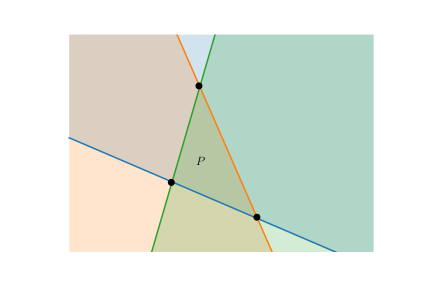
It is immediate from the definition that P⊂Rn is a polyhedron if and only if P is the intersection of k halfspaces in Rn for some k∈N. Figure 6.9 helps illustrate this idea.
Figure 6.9:A polyhedron P represented as intersecting halfspaces
An extreme point of a polyhedron P is a point p∈P that cannot be realized as the convex combination of other points in P. In other words, we cannot find two points x,y∈P that are distinct from p and satisfy λx+(1−λ)y=p for some λ∈[0,1]. The extreme points of P in Figure 6.9 are represented as black dots.
A cone in Rn is a set C⊂Rn such that x∈C implies αx∈C for all α>0.
A function g from a convex subset C of Rn to Rk is called convex if
g(λu+(1−λ)v)⩽λg(u)+(1−λ)g(v)whenever u,v∈C and 0⩽λ⩽1,
and concave if −g is convex. Concavity of g is obviously equivalent to
g(λu+(1−λ)v)⩾λg(u)+(1−λ)g(v)whenever u,v∈C and 0⩽λ⩽1.
When k=1, the function g is called, respectively, strictly convex or strictly concave if, in addition, the inequalities become strict whenever u,v are distinct and 0<λ<1.
These properties of functions are closely related to convexity of sets. For example, the same function g is convex if and only if its epigraph
epi(g):={(x,g(x))∈Rn+1:x∈C}
is convex.
In the next exercise, if {yi} is a finite collection of vectors in Rk, then maxiyi is the vector in Rk obtained by taking the maximum pointwise. The minimum miniyi is defined in a similar way.
Important examples of concave and convex scalar-valued functions include certain kinds of quadratic forms. For the following you should recall that a symmetric n×n matrix A is called
positive semidefinite if x⊤Ax⩾0 for any x in Rn,
positive definite if x⊤Ax>0 for any nonzero x in Rn,
negative semidefinite if x⊤Ax⩽0 for any x in Rn, and
negative definite if x⊤Ax<0 for any nonzero x in Rn.
It’s important to remember (but easy to forget) that symmetry is part of the definition of these properties. You probably remember that
A is positive definite (resp., semidefinite) if and only if all its eigenvalues are strictly positive (resp., nonnegative) and
A is positive definite (resp., semidefinite) ⟹ its determinant is strictly positive (resp., nonnegative).
The second statement follows from the first, since the determinant of a matrix equals the product of its eigenvalues.
The quadratic formq(x)=x⊤Ax is
convex if and only if A is positive semidefinite,
strictly convex if and only if A is positive definite,
concave if and only if A is negative semidefinite, and
strictly concave if and only if A is negative definite.
A number m contained in a subset A of R is called the maximum of A and we write m=maxA if a⩽m for every a∈A. It is called the minimum of A, written as m=minA, if m∈A and a⩾m for every a∈A.
Given an arbitrary set D and a function f:D→R, define
a maximizer of f on D if x∗∈D and f(x∗)⩾f(x) for all x∈D, and
a minimizer of f on D if x∗∈D and f(x∗)⩽f(x) for all x∈D.
Equivalently, x∗∈D is a maximizer of f on D if f(x∗)=maxx∈Df(x), and a minimizer if f(x∗)=minx∈Df(x). We define
x∈Dargmaxf(x):={x∗∈D:f(x∗)⩾f(x) for all x∈D}.
The set argminx∈Df(x) is defined analogously.
One important special case of part (ii) is that x∗∈D is a maximizer of f on D if and only if x∗ is a minimizer of −f on D. Hence, any maximization problem can be converted into a minimization problem and vice-versa.
Section 6.1.6.1 discussed existence of optimizers. In this section we consider uniqueness. The key observation is that, for convex and concave functions, local optimizers are global optimizers.
If C⊂Rn and f is a real-valued function on C, then u∗∈C is a local minimizer of f on C if there exists an open set G in C such that u∗∈G and f(u∗)⩽f(u) whenever u∈G. A local maximizer is defined analogously.
The next exercise highlights one of the most important facts concerning computation of solutions to optimization problems in real-world applications. It is especially valuable in high-dimensional settings, where optimization problems can be very challenging.
Similarly, if f is concave on C, then any local maximizer is a global maximizer.
If you have studied undergraduate economics, you will have used Lagrangian methods to solve constrained optimization problems. The objective of this section is to supply insight on when and why the method works, as well as to highlight the connection between an original constrained problem and a so-called “dual problem.” This connection yields deep insights in economics, finance, statistical learning, artificial intelligence and many other fields.
Here g maps E to Rm and h maps E to Rk. For example, the zero symbol in the statement g(x)=0 is a vector of zeros, and the meaning is that gi(x)=0 in R for i in 1,…,m. The interpretation of the second constraint is analogous.
Any x∈E that satisfies the constraints in (6.14) is called feasible. Let F(g,h) be the set of all feasible x∈E. A feasible point that attains the minimum in (6.14) is called optimal for—or a solution to—the optimization problem.
Our first claim is that the constrained optimization problem (6.14) is equivalent to the unconstrained problem
The first equality in (6.17) is by definition. The second two follow from (ii) and (i) respectively. Hence we need only verify (i)–(ii).
The function L in problem (6.16) is usually called the Lagrangian. The P in (6.15) stands for primal. So far we have shown that the original constrained problem and the primal problem are the same. The next step is to pair the primal problem with its dual problem, which is obtained by reversing the order of min and max in the primal:
The dual problem has two attractive features. One is that, when minimizing with respect to x, we do not need to concern ourselves with the constraints on x in the original formulation (6.14). The second is that, since L(x,θ) is linear in θ, and since we are minimizing a family of these functions with respect to x, the minimizer is a concave function. Concavity assists maximization, which is the next step in solving D.
The result D⩽P in Exercise 6.1.49 is called weak duality. If P=D, then strong duality is said to hold. Unlike weak duality, strong duality requires conditions on the primitives.
Evidently strong duality holds if and only if it is valid to reverse the order of the min and max operators in the definition of the primal (or the dual). Results of this kind are called min-max theorems. Such theorems hold at “saddle points” of the function L. The next section explains.
We seek necessary and sufficient conditions for strong duality, which will lead to a characterization of minimizers for the original constrained problem. To do so, we again take θ:=(λ,μ) and Θ:=Rm×R+k, so that
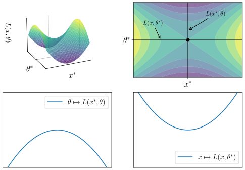
A depiction of a saddle point of a given bivariate function (x,θ)↦L(x,θ)∈R is given in Figure 6.10. The left hand side of the top panel is a 3D visualization, and the right hand side is a contour plot of the same function. The saddle point is at the center.
Figure 6.10:A saddle point (x∗,θ∗) of the function L
When the extrema in (6.20) exist, we have the following result:
Theorem 6.1.17 tells us that to solve the constrained optimization problem and establish strong duality, we need only obtain a saddle point of the Lagrangian.
For well behaved problems, saddle points can be identified via well known first-order conditions, called the Karush–Kuhn–Tucker (KKT) conditions. To state them, we return to the original problem (6.14) and write θ explicitly as (λ,μ), so that (x∗,λ∗,μ∗)∈E×Rm×R+k satisfies the saddle point condition if
L(x∗,λ,μ)⩽L(x∗,λ∗,μ∗)⩽L(x,λ∗,μ∗)for allx∈E,λ∈Rm and μ∈R+k.
The KKT conditions are met by (x∗,λ∗,μ∗)∈E×Rm×R+k if x∗∈F(g,h),
Here we are requiring that f,g,h are all differentiable at x∗ and, for a given function q:E→R, we use ∇ to represent the vector of partial derivatives. Equation (6.22) requires that the derivative of the Lagrangian with respect to x is zero at x∗. The second condition is called the complementary slackness condition.
The KKT conditions are nothing more than saddle point conditions. Condition (6.22) is the first order condition for an interior minimizer of the Lagrangian with respect to x, at the point (x∗,θ∗), which tries to identify the local minimum visualized in the lower right panel of Figure 6.10. The complementary slackness condition is also needed because if μi∗hi(x∗)=0 fails at some i, then μi∗hi(x∗)<0 must hold, in which case we could strictly increase the Lagrangian by shifting μi∗ to 0. This violates the saddle point property.
If enough regularity conditions hold, then the KKT conditions exactly identify extremal points. Here is one example, which is proved in Chapter 8 of Matousek & Gärtner (2007).
The notation x⩽y over vectors is standard, while x≪y is less so. In some fields, n≪k is used as an abbreviation for “n is much smaller than k.” Our usage lines up with most of the literature on partially ordered vector spaces. See, e.g., Zhang (2012).
This definition is not ambiguous because every possible enumeration leads to the same value when the absolute sum is finite (see, e.g., the rearrangement theorem in Bartle & Sherbert (2011), §9.1).
Hint: Start with the case ∣S∣=2. Argue that the case with n elements follows from this case and the ordinary (weak) triangle inequality ∣∑x∈Sg(x)∣⩽∑x∈S∣g(x)∣.