5 Nonlinear Interactions

Much of what makes network analysis interesting is how ramifications of choices flow across networks. In general, decisions made at a given node $i$ affect responses of neighboring nodes and, through them, neighbors of neighboring nodes, and so on. As these consequences flow across the network, they in turn affect choices at $i$. This is a tail-chasing scenario, which can be unraveled through fixed point theory.

In some network settings, such as the input-output model in Section 2.1, interactions are linear and fixed point problems reduce a system of linear equations. In other settings, interactions are inherently nonlinear and, as a result, we need more sophisticated fixed point theory.

This chapter is dedicated to the study of networks with nonlinear interactions. We begin with relevant fixed point theory and then apply it to a sequence of problems that arise in analysis of economic networks, including production models with supply constraints and financial networks.

5.1Fixed Point Theory¶

Let $S$ be any set. Recall from Section 6.1.1.6 that, given a self-map $G$ on $S$, a point $x \in S$ is called a fixed point of $G$ if $Gx = x$. (A self-map on $S$ is a function $G$ from $S$ to itself. When working with self-maps it is common to abbreviate $G(x)$ to $Gx$.) In this chapter, we will say that $G$ is globally stable on $S$ if $G$ has a unique fixed point $x^* \in S$ and $G^k x \to x^*$ as $k \to \infty$ for all $x \in S$. In other words, under this property, the fixed point is not only unique but also globally attracting under iteration of $G$.

We have already discussed fixed points, indirectly or directly, in multiple contexts:

• In Chapter 2 we studied the equation $x = A x + d$, where $x$ is an output vector, $A$ is a matrix of coefficients and $d$ is a demand vector. A solution $x$ to this equation can also be thought of as a fixed point of the affine map $Fx = Ax + d$.

• In Chapter 4 we learned that a stationary distribution of a finite Markov model with state space $S$ and adjacency matrix $P$ is a $\psi \in \dD(S)$ with $\psi = \psi P$. In other words, $\psi$ is a fixed point of $\psi \mapsto \psi P$ in $\dD(S)$.

• In Chapter 3 we studied the Bellman equation $q(x) = \min_{y \in \oO(x)} \{ c(x, y) + q(y) \}$ and introduced an operator the Bellman operator $T$, with the property that its fixed points exactly coincide with solutions to the Bellman equation.

In each case, when we introduced these fixed point problems, we immediately needed to consider questions of existence and uniqueness of fixed points. Now we address these same issues more systematically in an abstract setting.

5.1.1Contraction Mappings¶

In Chapter 2 we studied solutions of the system $x = Ax + b$ that are fixed points of the affine map $Fx = Ax + b$ on $\RR^n$ studied in Example 5.1.1. The Neumann series lemma is, in essence, a statement about existence and uniqueness of fixed points of this map. Here we investigate another fixed point theorem, due to Stefan Banach (1892–1945), that can be thought of as extending the Neumann series lemma to nonlinear systems.

5.1.1.1Contractions¶

Let $S$ be a nonempty subset of $\RR^n$. A self-map $F$ on $S$ is called contracting or a contraction of modulus $\lambda$ on $S$ if there exists a $\lambda < 1$ and a norm $\| \cdot \|$ on $\RR^n$ such that

The next example uses a similar idea but is based on a different norm.

Consider again Example 5.1.1. For the affine map $Fx = Ax + b$, the condition $\| A \| < 1$ used to obtain contraction is stronger than the condition $r(A) < 1$ used to obtain a unique fixed point in the Neumann series lemma (see Exercise 2.3.11). Furthermore, the Neumann series lemma provides a geometric series representation of the fixed point. On the other hand, as we now show, the contraction property can be used to obtain unique fixed points when the map in question is not affine.

5.1.1.2Banach’s Theorem¶

The fundamental importance of contractions stems from the following theorem.

We complete a proof of Theorem 5.1.1 in stages.

5.1.1.3Eventual Contractions¶

Let $S$ be a nonempty subset of $\RR^n$. A self-map $F$ on $S$ is called eventually contracting if there exists a $k \in \NN$ such that $F^k$ is a contraction on $S$. Significantly, most of the conclusions of Banach’s theorem carry over to the case where $F$ is eventually contracting.

There is a close connection between Theorem 5.1.2 and the Neumann series lemma (NSL). If $S=\RR^n$ and $F x = A x + b$ with $r(A) < 1$, then the NSL implies a unique fixed point. We can also obtain this result from Theorem 5.1.2, since, for any $k \in \NN$,

As $r(A) < 1$, we can choose $k$ such that $\| A^k \| < 1$ (see Section 2.3.3). Hence $F$ is eventually contracting and Theorem 5.1.2 applies.

As mentioned above, contractions and eventual contractions have much wider scope than the NSL, since they can also be applied in nonlinear settings. At the same time, the NSL is preferred when its conditions hold, since it also gives inverse and power series representations of the fixed point.

5.1.1.4A Condition for Eventual Contractions¶

The result below provides a useful test for the eventual contraction property. (In the statement, the absolute value of a vector is defined pointwise, as in Section 6.1.2.2.)

5.1.2Shortest Paths Revisited¶

Consider again the shortest path problem introduced in Section 3.1. One modification that sometimes appears in applications is the addition of discounting during travel between vertices. For example, if the vertices are international ports and travel takes place by sea, then port-to-port travel time is measured in weeks or even months. It is natural to apply time discounting to future costs associated with that travel, to implement the idea that paying a given dollar amount in the future is preferable to paying it now.

Recall that, without discounting, the Bellman equation for the shortest path problem takes the form $q(x) = \min_{y \in \oO(x)} \{ c(x, y) + q(y) \}$ for all $x \in V$, where $c$ is the cost function $V$ is the set of vertices and $q$ is a candidate for the cost-to-go function. We showed that the minimum cost-to-go function $q^*$ satisfies the Bellman equation and is the unique fixed point of the Bellman operator.

The Bellman equation neatly divides the problem into current costs, embedded in the term $c(x, y)$, and future costs embedded in $q(y)$. To add discounting, we need only discount $q(y)$. We do this by multiplying it by a discount factor $\beta \in (0, 1)$. The Bellman equation is then $q(x) = \min_{y \in \oO(x)} \{ c(x, y) + \beta q(y) \}$ for all $x \in V$ and the Bellman operator is

In Section 3.1.2, without discounting, we had to work hard to show that the Bellman operator has a unique fixed point in $U$, the set of all $q \colon V \to \RR_+$ with $q(d)=0$. With discounting the proof is easier, since we can leverage the Banach contraction mapping theorem.

In what follows, we identify the vertices in $V$ with integers $1, \ldots, n$, where $d$ is identified with $n$. We then understand $U$ as all nonnegative vectors $q$ in $\RR^n$ with $q(n) = 0$. (We continue to write $q(x)$ for the $x$-th element of the vector $q$, but now $x$ is in $\natset{n}$.)

Now let $\| \cdot \|_\infty$ be the supremum norm on $\RR^n$ (see Section 2.3.1). We claim that $T$ is a contraction on $U$ of modulus $\beta$. To see that this is so, fix $p, q \in U$ and observe that, pointwise,

where the first inequality is by the order-preserving of $T$ and the second follows from Exercise 5.1.9. Hence

Reversing the roles of $p$ and $q$ gives the reverse inequality. Hence

for all $x \in \natset{n}$. Taking the maximum on the left hand side yields $\|Tq - Tp \|_\infty \leq \beta \|q - p\|_\infty$, which shows that $T$ is a contraction of modulus $\beta$. Hence Banach’s theorem applies and a unique fixed point exists.

5.1.3Supply Constraints¶

While the input-output model from Section 2.1.2 has many useful applications, its linear structure can be a liability. One natural objection to linearity is supply constraints: if sector $j$ doubles its orders from sector $i$, we cannot always expect that sector $i$ will quickly meet this jump in demand.

In this sector we investigate the impact of supply constraints on equilibrium. These constraints introduce nonlinear relationships between nodes that affect equilibria and make analysis more challenging.

We recall from Section 2.1.2 that $d_i$ is final demand for good $i$, $x_i$ is total sales of sector $i$, $z_{ij}$ is inter-industry sales from sector $i$ to sector $j$, and $a_{ij} = z_{ij}/x_j$ is dollar value of inputs from $i$ per dollar output from $j$.

Departing from our previous formulation of equilibrium in the input-output model, suppose that, in the short run, the total output value of sector $i$ is constrained by positive constant $\bar x(i)$. Holding prices fixed (in the short run), this means that sector $i$ has a capacity constraint in terms of unit output. For the purposes of our model, the vector of capacity constraints $\bar x := (\bar x(i))_{i=1}^n$ can be any vector in $\RR^n_+$.

For each sector $i$, we modify the accounting identity (2.1) to

where $o_{ij}$ is the value of orders from sector $i$ made by sector $j$. Thus, if the capacity constraint in sector $i$ is not binding, then output is the sum of orders from other sectors and orders from final consumers. If $\bar x(i)$ is less than this sum, however, then sector $i$ produces to capacity $\bar x(i)$.

An equilibrium for this model is one where all orders are met, subject to capacity constraints. The fact that orders are met means that $o_{ij} = z_{ij} = a_{ij} x_j$. Substituting this equality into (5.6) and rewriting as a vector equality, (5.6) can equivalently be formulated as

The following exercise is key to solving the fixed point problem (5.7).

We are now ready to prove existence of a unique fixed point under the assumption that every sector has positive value added.

5.1.4Fixed Points and Monotonicity¶

Banach’s fixed point theorem and its extensions are foundations of many central results in pure and applied mathematics. For our purposes, however, we need to search a little further, since not all mappings generated by network models have the contraction property. In this section, we investigate two fixed point results that drop contractivity in favor of monotonicity.

5.1.4.1Existence¶

Without contractivity, one needs to work harder to obtain even existence of fixed points, let alone uniqueness and convergence. This is especially true if the map in question fails to be continuous. If, however, the map is order preserving, then existence can often be obtained via some variation on the Knaster–Tarski fixed point theorem.

Here we present a version of this existence result that is optimized to our setting, while avoiding unnecessary excursions into order theory. In stating the theorem, we recall that a closed order interval in $\RR^n$ is a set of the form

where $a$ and $b$ are vectors in $\RR^n$. Also, we call $(x_k) \subset \RR^n$ increasing (resp., decreasing) if $x_k \leq x_{k+1}$ (resp., $x_k \geq x_{k+1}$) for all $k$.

For a self-map $G$ on $S \subset \RR^n$, we say that $x^*$ is a least fixed point (resp., greatest fixed point) of $G$ on $S$ if $x^*$ is a fixed point of $G$ in $S$ and $x^* \leq x$ (resp., $x \leq x^*$) for every fixed point $x$ of $G$ in $S$. Finally, we say that $G$ is

• continuous from below if $x_k \uparrow x$ in $S$ implies $G x_k \uparrow G x$ in $S$.

• continuous from above if $x_k \downarrow x$ in $S$ implies $G x_k \downarrow G x$ in $S$.

Here $x_k \uparrow x$ means that $(x_k)$ is increasing and $x_k \to x$. The definition of $x_k \downarrow x$ is analogous. In the next theorem, $S := [a, b]$ is a closed order interval in $\RR^n$ and $G$ is a self-map on $S$.

5.1.4.2Du’s Theorem¶

Theorem 5.1.5 is useful because of its relatively weak assumptions. At the same time, it fails to deliver uniqueness. Hence its conclusions are considerably weaker than the results we obtained from contractivity assumptions in Section 5.1.1.

In order to recover uniqueness without imposing contractivity, we now consider order-preserving maps that have additional shape properties. In doing so, we use the definition of concave and convex functions in Section 6.1.5.2.

A proof of Theorem 5.1.6 was obtained in an more abstract setting in Du (1990). Interested readers can consult that article for a proof.

To illustrate how these results can be applied, consider the constrained production model without assuming positive value added, so that $r(A) < 1$ is not enforced. In Exercise 5.1.12 we obtained existence. With Theorem 5.1.6 in hand, we can also show uniqueness whenever $d \gg 0$ and $\bar x \gg 0$.

Indeed, we have already seen that $G$ is a self-map on $S := [0, \bar x]$ and, when this last condition holds, we have $G 0 = d \wedge \bar x \gg 0$. Hence the conclusions of Theorem 5.1.6 will hold if we can establish that $G$ is concave.

Here is a small extension of Du’s theorem that will prove useful soon:

5.2Financial Networks¶

Given the long history of crises in financial markets around the globe, economists and business analysts have developed many tools for assessing the credit-worthiness of banks and other financial institutions. After the major financial crises of 2007-2008, originating in the subprime market in the US and the sudden collapse of Lehmann Brothers, it became clear that the financial health of individual institutions cannot be assessed in isolation. Rather, it is essential to analyze solvency and credit-worthiness in terms of the entire network of claims and liabilities within a highly interconnected financial system. In this section, we review financial crises and apply network analysis to study how they evolve.

5.2.1Contagion¶

Some financial crises have obvious causes external to the banking sector. A prominent example is the hyperinflation that occurred in Weimar Germany around 1921–1923, which was driven by mass printing of bank notes to meet war reparations imposed under the Treaty of Versailles. Here the monetary authority played the central role, while the actions of private banks were more passive.

Other crises seem to form within the financial sector itself, driven by interactions between banks, hedge funds, and asset markets. In many cases, the crisis follows a boom, where asset prices rise and economic growth is strong. Typically, the seeds of the crisis are laid during this boom phase, when banks extend loans and firms raise capital on the basis of progressively more speculative business plans. At some point it becomes clear to investors that these businesses will fail to meet expectations, leading to a rush for the exit.

The last phase of this cycle is painful for the financial sector, since rapidly falling asset values force banks and other financial institutions to generate short-term capital by liquidating long-term loans, typically with large losses, as well as selling assets in the face of falling prices, hoarding cash and refusing to roll over or extend short term loans to other institutions in the financial sector. The financial crisis of 2007–2008 provides a textbook example of these dynamics.

One key aspect of the financial crisis of 2007–2008, as well as other similar crises, is contagion, which refers to the way that financial stress spreads across a network of financial institutions. If one institution becomes stressed, that stress will often spread to investors or counterparties to which this institution is indebted. The result of this process is not easy to predict, since, like equilibrium in the production networks studied in Chapter 2, there is a tail chasing problem: stress spreads from institution $A$ to institutions $B$, $C$ and $D$, which may in turn increase stress on $A$, and so on.

In this section we study financial contagion, beginning with a now-standard model of default cascades.

5.2.2Default Cascades¶

Default cascades are a form of financial contagion, in which default by a node in a network leads to default by some of its counterparties, which then spreads across the network. Below we present a model of default cascades and analyze its equilibria.

5.2.2.1Network Valuation¶

Consider a financial network $\gG = (V, E, w)$, where $V = \natset{n}$ is a list of $n$ financial institutions called banks, with an edge $(i, j) \in E$ indicating that $j$ has extended credit to $i$. The size of that loan is $w(i, j)$. Thus, an edge points in the direction of a liability, as in Figure 1.17: edge $(i, j)$ indicates a liability for $i$ and an asset for $j$. As in Section 1.4.1, the set of all direct predecessors of $i \in V$ will be written as $\iI(i)$, while the set of all direct successors will be denoted $\oO(i)$.

Banks in the network have both internal and external liabilities, as well as internal and external assets. Internal (i.e., interbank) liabilities and assets are given by the weight function $w$, in the sense that $w(i,j)$ is a liability for $i$, equal to the size of its loan from $j$, and also an asset for $j$. Positive weights indicate the presence of counterparty risk: when $j$ holds an asset of book value $w(i, j)$, whether or not the loan is repaid in full depends on the stress placed on bank $i$ and rules that govern repayment in the event of insolvency.

We use the following notation for the primitives of the model: $x_i := \sum_{j \in \oO(i)} w(i, j)$ is total interbank liabilities of bank $i$,

is the matrix of relative interbank liabilities, $a_i$ is external assets held by bank $i$ and $d_i$ is external liabilities.

When considering the interbank assets of bank $j$, we need to distinguish between the book value $\sum_{i \in \iI(j)} w(i, j)$ of its claims on other banks and the realized value in the face of partial or complete default by its counterparties $\iI(j)$. To this end, we introduce a clearing vector $p \in \RR^n_+$, which is a list of proposed payments by each bank in the network. In particular, $p_i$ is total payments made by bank $i$ to its counterparties within the banking sector. Under the choice of a particular clearing vector, the actual payments received by bank $j$ on its internal loan portfolio are $\sum_{i \in V} p_i \Pi_{ij}$.

The last statement is an assumption about the legal framework for the banking sector. It means that the actual payment $p_i \Pi_{ij}$ from $i$ to $j$ is proportional to the amount that $i$ owes $j$, relative to its total interbank obligations. The idea is that all counterparties in the banking sector have equal seniority, so that residual funds are spread across claimants according to the relative size of the claims.

Let $\hat p_j$ be the amount of funds bank $j$ makes available to repay all of its debts, both interbank and external. This quantity is

The right hand term inside the $\min$ operator is total debts of bank $j$. The left hand side is the amount on hand to repay those debts, including external assets and repayments by other banks. The bank repays up to—but not beyond—its ability to pay.

External liabilities are assumed to be senior to interbank liabilities, which means that for bank $j$ we also have

Thus, interbank payments by $j$ are a remainder after external debts are settled. If these debts exceed the bank’s ability to pay, the bank becomes insolvent and pays nothing to internal creditors. This is a form of limited liability.

Combining (5.10) and (5.11) and rearranging slightly yields

Now let’s take $p$, $a$, $d$ and $x$ as row vectors in $\RR^n$ and write this collection of equations, indexed of $j$, in vector form. With $\max$ and $\min$ taken pointwise, and using the symbols $\vee$ and $\wedge$ for max and min, we get

A solution to this equation is called an equilibrium clearing vector for the banking system.

5.2.2.2Existence and Uniqueness of Fixed Points¶

In order to analyze existence and uniqueness of equilibria, we introduce the operator $T \colon \RR^n \to \RR^n$ defined by

where $e := a - d$ represents net external assets. Evidently $p \in \RR^n_+$ is an equilibrium clearing vector if and only if it is a fixed point of $T$.

Using this operator, establishing existence of at least one equilibrium clearing vector is not problematic for this model, regardless of the values of the primitives and configuration of the network:

While existence is automatic in this model, uniqueness is not:

There are several approaches to proving uniqueness of fixed points of $T$. Here is one:

This leads us to the following result:

There are several possible assumptions about the structure of the bank network $\gG$ that imply the conditions of Proposition 5.2.1. For example, it would be enough that $\gG$ is strongly connected and has at least one bank with zero interbank liabilities. Below we investigate another sufficient condition, related to cyclicality.

5.2.2.3Nonnegative External Equity¶

In this section we investigate the special case in which

(E1) each bank has nonzero interbank debt, so that $\Pi$ is a stochastic matrix, and

(E2) external net assets are nonnegative, in the sense that $e = a - d \geq 0$.

In view of (E1), we cannot hope to use Proposition 5.2.1, since we always have $r(\Pi)=1$ when $\Pi$ is stochastic. Nonetheless, we can still obtain global stability under certain restrictions on $e$ and the topology of the network. Here is a relatively straightforward example, which we will later try to refine:

The condition $e \gg 0$ is rather strict. Fortunately, it turns out that we can obtain global stability under significantly weaker conditions. To this end, we will say that node $j$ in a financial system $\gG$, is cash accessible if there exists an $i \in V$ such that $i \to j$ and $e(i) > 0$. In other words, $j$ is downstream in the liability chain from at least one bank with positive net assets outside of the banking sector.

With the result from Exercise 5.2.6 in hand, the next lemma is easy to establish.

Stronger results are available, with a small amount of effort. In fact, under (E1)–(E2), there is a strong sense in which uniqueness of the fixed point is obtained without any further assumptions, provided that we rule out an ambiguity related to what happens when $e=0$. That ambiguity is discussed in the next exercise and further references can be found in Section 5.3.

Although Exercise 5.2.7 suggests ambiguity about outcomes when $e = 0$, it is natural to adopt the convention that the equilibrium clearing vector $p^*$ obeys $p^*=0$ whenever $e=0$. If the entire banking sector has no zero net assets, then no positive payment sequence can be initiated (without outside capital).

In the next exercise, we say that $U \subset V$ is accessible from $i \in V$ if there exists a $j \in U$ such that $j$ is accessible from $i$.

5.2.3Equity-Cross Holdings¶

In this section we analyze the model of default cascades constructed by Elliott et al., 2014. The model differs from the one studied in Section 5.2.2 in several ways. One is that financial institutions are linked by share cross-holdings: firm $i$ owns a fraction $c_{ij}$ of firm $j$ for $i, j \in V := \natset{n}$. This implies that failure of firm $j$ reduces the market value of firm $i$, which in turn reduces the market value of other firms, and so on.

The second—and ultimately more significant—difference is the introduction of failure costs that add significant nonlinearities to the model. Failure costs reinforce the impact of each firm failure, leading to greater shock propagation across the network. This feature ties into the intuitive idea that, when many firms are financially stressed, a failure by one firm can trigger a wave of bankruptcies.

5.2.3.1Book and Market Value¶

We now describe the features of the model. Let $C = (c_{ij})_{i, j \in V}$ be the matrix of fractional cross-holdings, as mentioned above, with $0 \leq c_{ij} \leq 1$ for all $i,j$.

Assumption 5.2.1 implies that firms are not solely owned by other firms in the network: investors outside the network hold at least some fraction of firm $i$ for all $i$.

The book value of firm $i$ is given by

Here the first term $e_i \geq 0$ is external assets of firm $i$ and the second represents the value of firm $i$’s cross-holdings. In vector form, the last equation becomes $b = e + C b$.

There is a widely used argument that cross-holdings artificially inflate the value of firms, in the sense that the sum of book values of firms exceeds $\sum_i e_i$, the sum of underlying equity values. The next exercise illustrates:

Due to this artificial inflation, we distinguish between the book value $b_i$ of a firm and its market value $\bar v_i$, which is defined as $r_i b_i$ with $r_i := 1 - \sum_{k} c_{ki}$. The value $r_i$, which gives the share of firm $i$ held by outsider investors, is strictly positive for all $i$ by Assumption 5.2.1. With $R := \diag(r_1, \ldots, r_n)$, we can write the vector of market values as $\bar v = R b$. Substituting in (5.16) gives

5.2.3.2Failure Costs¶

So far the model is very straightforward, with the market value of firms being linear in external assets $e$. However, since bankruptcy proceedings are expensive, it is reasonable to assume that firm failures are costly. Moreover, when the market value of a firm falls significantly, the firm will experience difficulty raising short term funds, and will often need to cease revenue generating activities and sell illiquid assets well below their potential value.

We now introduce failure costs. As before, $\bar v_i$ is market value without failure costs, as determined in (5.17), while $v_i$ will represent market value in the presence of failure costs. Failure costs for firm $i$ are modeled as a threshold function

where $\theta \in (0, 1)$ and $\beta > 0$ are parameters. Thus, costs are zero when $v_i$ is large and $-\beta$ when they fall below the threshold $\theta \bar v_i$. In particular, a discrete failure cost of $-\beta$ is incurred when firm value falls far enough below the no-failure market value $\bar v_i$. The larger is $\theta$, more prone firms are to failure.

The book value of firm $i$ without failure costs was defined in (5.15). The book value of firm $i$ in the presence of failure costs is defined as

Written in vector form, with $f$ applied pointwise to the vector $v$, we get $b = e + C b - f (v)$. Solving for $b$ gives $b = (I-C)^{-1} (e - f (v))$. The corresponding market value is

Notice that, when no firms fail, we have $v_i = \bar v_i$, as expected.

5.2.3.3Equilibria¶

Equation (5.18) is a nonlinear equation in $n$ unknowns. A vector $v \in \RR^n$ solves (5.18) if and only if it is a fixed point of the operator $T \colon \RR^n \to \RR^n$ defined by

In what follows we set $d := A(e - \beta \1)$ and $S := [d, \bar v]$.

Note that $v^* = v^{**}$ is a possibility, in which case $T$ has a unique fixed point in $S$.

Why does $(T^k d)_{k \in \NN}$ converge up to $v^*$ in a finite number of steps? First, as you saw in the solution to Exercise 5.2.12, the map $T$ is an order-preserving self-map on $[d, \bar v]$, so $Td \in [d, \bar v]$. In particular, $d \leq Td$. Iterating on this inequality and using the order-preserving property gives $d \leq Td \leq T^2 d \leq \cdots$, so $(T^k d)$ is indeed increasing. Moreover, the range of $T$ is a finite set, corresponding to all vectors of the form

where $w$ is an $n$-vector containing only zeros and ones. Finiteness holds because there are only finitely many binary sequences of length $n$.

Similar logic can be applied to prove that $(T^k \bar v)_{k \in \NN}$ converges down to $v^{**}$ in a finite number of steps.

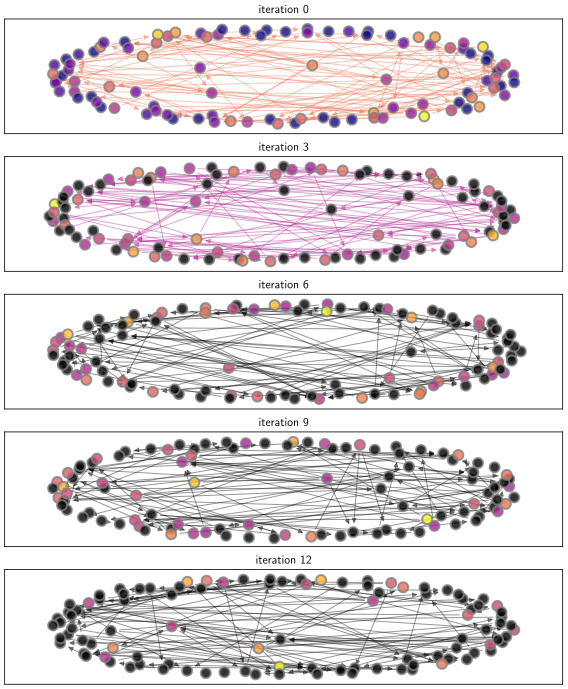
If we set $v^0 = \bar v$ and $v^{k+1} = T v^k$, we can consider the sequence of valuations $(v^k)$ as a dynamic process, and the number of currently failing firms $m^k := \sum_i \1\{v^k_i < \theta\}$ can be understood as tracking waves of bankruptcies. Failures of firms in the first wave put stress on otherwise healthy firms that have exposure to the failed firms, which in turn causes further failures and so on.

As discussed in Proposition 5.2.3, the sequence $(v^k)$, which can also be written as $(T^k \bar v)$, is decreasing pointwise. In other words, the value of each firm is non-increasing. Hence, if $v^k_i < \theta$ for some $k$, then $v^{k+j}_i < \theta$ for all $j \geq 0$.

Figure 5.1 illustrates a growing wave of failures that can arise in a financial network. Firms with lighter colors have better balance sheets. Black firms have failed. The code for generating this figure, along with details on parameters, can be found in the code book.

5.3Chapter Notes¶

Shin (2010) gives an excellent overview of systemic risk and the financial crisis of 2007–2008. Battiston et al. (2012) study connectedness in financial networks and introduce a measure of systemic impact called DebtRank. Bardoscia et al. (2015) provide a dynamic theory of instability related to DebtRank. Demange (2018) provides a threat index for contagion in financial networks related to Katz centrality. Bardoscia et al. (2019) analyze risks associated with solvency contagion during crises. Jackson & Pernoud (2019) study investment in risky portfolios by banks in financial networks with debt and equity interdependencies. Jackson & Pernoud (2020) analyze optimal bailouts in financial networks. Amini & Minca (2020) offer an introduction to modeling of clearing systems, analyzing equilibria for network payments and asset prices. Jackson & Pernoud (2021) provide a survey of the relationship between financial networks and systemic risk.

The setting in Section 5.2.2.3 was investigated by Eisenberg & Noe (2001), one of the first papers on a network approach to default cascades. Additional details on stability properties can be found in Stachurski (2022). As already mentioned, Section 5.2.3 is based on Elliott et al., 2014, which also includes an interesting discussion of how the level of integration across a network affects equilibria. Klages-Mundt & Minca (2021) discuss optimal intervention in economic networks via influence maximization methods, using Elliott et al. (2014) as an example. Acemoglu et al. (2021) study how anticipation of future defaults can result in "credit freezes."

A general discussion of contraction maps and related fixed point theory can be found in Goebel & Kirk (1990) and Cheney (2013). For more on fixed point methods for order preserving operators, see, for example, Guo et al. (2004), Zhang (2012), Marinacci & Montrucchio (2019) or Deplano et al. (2020).