In this chapter we study production in multisector environments. The basic framework is input-output analysis, which was initiated by Wassily Leontief (1905–1999) and popularized in Leontief (1941). Input-output analysis is routinely used to organize national accounts and study inter-industry relationships. In 1973, Leontief received the Nobel Prize in Economic Sciences for his work on input-output systems.
Input-output analysis is currently being incorporated into modern theories of trade, growth, shock propagation and aggregate fluctuations in multisector models (Section 2.4 provides a detailed list of references). One of the reasons for renewed interest is that the introduction of concepts from network analysis and graph theory has yielded new insights. This chapter provides an introduction to the main ideas.
2.1Multisector Models
In this section we introduce the basic input output model, explain the network interpretation of the model, and connect traditional questions, such as the relative impact of demand shocks across sectors, to network topology and network centrality.
2.1.1Production Networks
We begin with the foundational concepts of input-output tables and how they relate to production networks. To simplify the exposition, we ignore imports and exports in what follows. (References for the general case are discussed in Section 2.4.)
2.1.1.1Input-Output Analysis
Agencies tasked with gathering national and regional production accounts (such as the US Bureau of Economic Analysis) compile input-output data based on the structure set out by Leontief (1941). Firms are divided across sectors, each of which produces a single homogeneous good. These sectors are organized into an input-output table, a highly simplified example of which is
| sector 1 | sector 2 | sector 3 | |
|---|---|---|---|
| sector 1 | |||
| sector 2 | |||
| sector 3 |
Entries are called the input-output coefficients;
Thus, is large if sector is an important supplier of intermediate goods to sector . The sum of the -th column of the table gives the value of all inputs to sector . The -th row shows how intensively each sector uses good as an intermediate good.
The production coefficient matrix induces a weighted digraph , where is the list of sectors and
is the edge set. The values show backward linkages across sectors.
Given , the set of direct successors of is all sectors to which supplies a positive quantity of output. The set is all sectors that supply a positive quantity to .
Figure 2.1 illustrates the weighted digraph associated with the 15 sector version of the input-output tables provided by the Bureau of Economic Analysis for the year 2021.[1] An arrow from to indicates a positive weight . Weights are indicated by the widths of the arrows, which are proportional to the corresponding input-output coefficients. The sector codes are provided in Table 2.1. The size of vertices is proportional to their share of total sales across all sectors.
A quick look at Figure 2.1 shows that manufacturing (ma) is an important supplier for many sectors, including construction (co) and agriculture (ag). Similarly, the financial sector (fi) and professional services (pr) supply services to a broad range of sectors. On the other hand, education (ed) is relatively downstream and only a minor supplier of intermediate goods to other sectors.
The color scheme for the nodes is by hub-based eigenvector centrality, with hotter colors indicating higher centrality. Later, in Section 2.1.3 we will give an interpretation of hub-based eigenvector centrality for this setting that connects to relative impact of demand shocks.
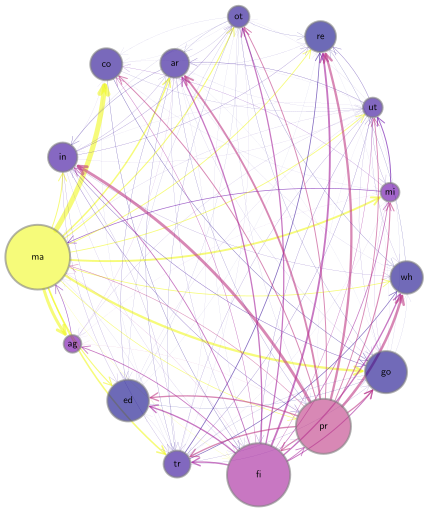
Figure 2.1:Backward linkages for 15 US sectors in 2021
Table 2.1:Sector codes for the 15 good case
| Label | Sector |
|---|---|
| ag | Agriculture, forestry, fishing, and hunting |
| mi | Mining |
| ut | Utilities |
| co | Construction |
| ma | Manufacturing |
| wh | Wholesale trade |
| re | Retail trade |
| tr | Transportation and warehousing |
| in | Information |
| fi | Finance, insurance, real estate, rental, and leasing |
| pr | Professional and business services |
| ed | Educational services, health care, and social assistance |
| ar | Arts, entertainment, accommodation, and food services |
| ot | Other services, except government |
| go | Government |
2.1.1.2Connectedness
We will gain insights into input-output networks by applying some of the graph-theoretic notions studied in Section 1.4. One elementary property we can investigate is connectedness. We can imagine that demand and productivity shocks diffuse more widely through a given production network when the network is relatively connected. Conversely, the impact of a demand shock occurring within an absorbing set will be isolated to sectors in that set.
The 15 sector network in Figure 2.1 is strongly connected. Checking this visually is hard, so instead we use a graph-theoretic algorithm that finds strongly connected components from QuantEcon’s DiGraph class. (This class is convenient for the current problem because instances are created directly from the adjacency matrix.) Examining the attributes of this class when the weights are given by the 15 sector input-output model confirms its strong connectedness. The same class can be used to verify that the network is also aperiodic. Hence, the input-output matrix is primitive. This fact will be used in computations below.
2.1.1.3Disaggregation
Figure 2.2 repeats the graphical representation for the more disaggregated 71 sector case. Sector codes are provided in Table 2.2. Input-output coefficients below were rounded to zero to increase visual clarity. As in the 15 sector case, the size of vertices and edges is proportional to share of sales and input-output coefficients respectively. Hotter colors indicate higher hub-based eigenvector centrality (which we link to propagation of demand shocks in Section 2.1.3).
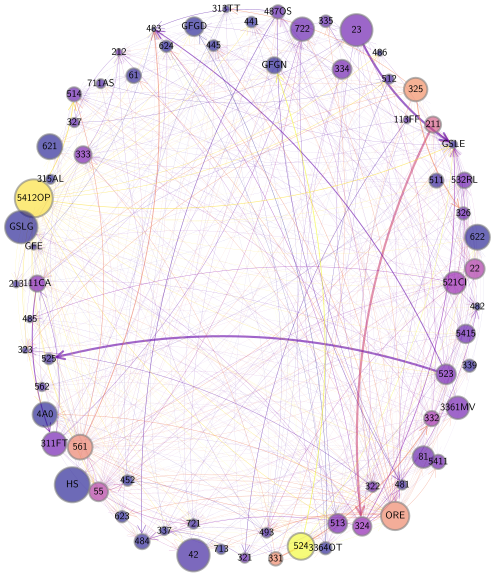
Figure 2.2:Network for 71 US sectors in 2021
Table 2.2:Sector codes for the 71 good case
| IO Code | Sector | IO Code | Sector |
|---|---|---|---|
| 111CA | Farms | 486 | Pipeline transportation |
| 113FF | Forestry, fishing | 487OS | Other transportation |
| 211 | Oil and gas extraction | 493 | Warehousing and storage |
| 212 | Mining, except oil, gas | 511 | Publishing industries |
| 213 | Mining support activities | 512 | Motion picture and sound |
| 22 | Utilities | 513 | Broadcasting, telecommunications |
| 23 | Construction | 514 | Data processing, internet publishing |
| 321 | Wood products | 521CI | Reserve banks, credit intermediation |
| 327 | Nonmetallic mineral products | 523 | Securities and investments |
| 331 | Primary metals | 524 | Insurance carriers |
| 334 | Computer & electronic products | 525 | Funds, trusts, financial vehicles |
| 333 | Machinery | HS | Housing |
| 332 | Fabricated metal products | ORE | Other real estate |
| 335 | Electrical equipment | 532RL | Rental and leasing services |
| 337 | Furniture | 55 | Firm management |
| 3364OT | Other transportation equipment | 5415 | Computer systems design |
| 3361MV | Motor vehicles, parts | 5412OP | Miscellaneous technical services |
| 339 | Miscellaneous manufacturing | 5411 | Legal services |
| 311FT | Food, beverage, tobacco | 561 | Administrative |
| 313TT | Textile mills and products | 562 | Waste management |
| 315AL | Apparel and leather | 61 | Educational services |
| 322 | Paper products | 621 | Ambulatory health care services |
| 323 | Printing | 622 | Hospitals |
| 324 | Petroleum and coal | 623 | Nursing and residential care facilities |
| coal products | residential care facilities | ||
| 325 | Chemical products | 624 | Social assistance |
| 326 | Plastics, rubber | 711AS | Arts, spectator sports, museums |
| 42 | Wholesale trade | 713 | Amusements, gambling, recreation |
| 441 | Motor vehicle and parts dealers | 721 | Accommodation |
| 445 | Food and beverage stores | 722 | Food services and drinking places |
| 452 | General merchandise stores | 81 | Other services, except government |
| 4A0 | Other retail | GFGD | Federal government (defense) |
| 481 | Air transportation | GSLE | State and local government enterprises |
| 482 | Rail transportation | GFE | Federal government enterprises |
| 483 | Water transportation | GSLG | State and local government |
| 484 | Truck transportation | GFGN | Federal government (nondefense) |
| 485 | Passenger transportation |
Unlike the 15 sector case, the 71 sector 2021 input-output matrix is not strongly connected. This is because it contains sinks (sectors with zero out-degree). For example, according to the data, 441 “motor vehicle and parts dealers” do not supply any intermediate inputs, although they do of course supply products to final consumers.
2.1.2Equilibrium
Equilibrium in Leontief models involves tracing the impact of final demand as it flows backward through different sectors in the economy. To illustrate the challenges this generates, consider the simplified network shown in Figure 2.3. Suppose sector 3 receives a positive demand shock. Meeting this demand will require greater output from its immediate suppliers, which are sectors 2 and 4. However, an increase in production in sector 2 requires more output from sector 1, which then requires more output from sector 3, where the initial shock occurred. This, in turn, requires more output from sectors 2 and 4, and so on. Thus, the chain of backward linkages leads to an infinite loop. Resolving this tail chasing problem requires some analysis.
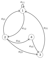
Figure 2.3:A simple production network
2.1.2.1Identities
To start our search for equilibria, we set
final consumer demand for good .
total sales of sector .
inter-industry sales from sector to sector .
All numbers are understood to be in units of national currency—dollars, say. For each sector we have the accounting identity
which states that total sales are divided between sales to other industries and sales to final consumers.
Notice that
where the values are the the input-output coefficients discussed in Section 2.1.1.1. Using the coefficients, (2.1) can be rewritten as
The first term on the right hand side is the amount of good required as inputs when the output vector is . We can combine the equations in (2.3) into the linear system
2.1.2.2Existence and Uniqueness
So far we have used no more than accounting identities and definitions. However, we would also like to use (2.4) to determine output vector given demand vector , taking as fixed. As a first step, we seek conditions under which nonnegative solutions to (2.4) exist and are unique.
The value added of sector is defined as sales minus spending on intermediate goods, or
Exercise 2.1.1 shows that Assumption 2.1.1 is very mild. For example, in a competitive equilibrium, where firms make zero profits, positive value added means that payments to factors of production other than intermediate goods (labor, land, etc.) are strictly positive.
The matrix in (2.6) is called the Leontief inverse associated with the coefficient matrix . We discuss its interpretation in Section 2.1.3.
2.1.2.3Assumptions
It is common to interpret the expression from (2.6) as meaning that supply is driven by demand. While this is not a universal truth, it does have plausibility in some settings, such as when analyzing demand shifts in the short run. Changes in demand lead to changes in inventories, which typically cause firms to modify production quantities. We investigate these ideas in depth in Section 2.1.3.
Another assumption concerns the production function in each sector. You might recall from elementary microeconomics that the Leontief production function takes the form
Here is output in a given sector, is a set of parameters and is a set of inputs. To understand why (2.7) is called a Leontief production function, note that by (2.2) we have
If we interpret for all , then (2.8) implies . This is a version of (2.7) specialized to sector . Hence (2.7) arises naturally from Leontief input-output analysis.
A final comment on assumptions is that, while the Leontief model is too simple for some purposes, it serves as a useful building block for more sophisticated models. We discuss one such model in Section 2.2.1.
2.1.3Demand Shocks
In this section we study impacts of changes in demand via a power series representation of the Leontief inverse . We assume throughout that , so that the series and are finite and equal.
2.1.3.1Response to Demand Shocks
Consider the impact of a demand shock of size , so that demand shifts from to . The equilibrium output vector shifts from to . Subtracting the first of these equations from the second and expressing the result in terms of differences gives . Using the geometric sum version of the Leontief inverse yields
The sums in this term show how the shock propagates backward through the production network:
is the initial response in each sector,
is the response generated by the first round of backward linkages,
is the response generated by the second round, and so on.
The total response is the sum of responses at all rounds.
We can summarize the above by stating that a typical element of shows the total impact on sector of a unit change in demand for good , after taking into account all direct and indirect effects. itself is reminiscent of a Keynesian multiplier: changes in demand are multiplied by this matrix to generate final output.
Figure 2.4 helps visualize the Leontief inverse computed from the 15 sector network. Hotter colors indicate larger values for , with on the vertical axis and on the horizontal axis. We see, for example, that an increase in demand in almost any sector generates a rise in manufacturing output.
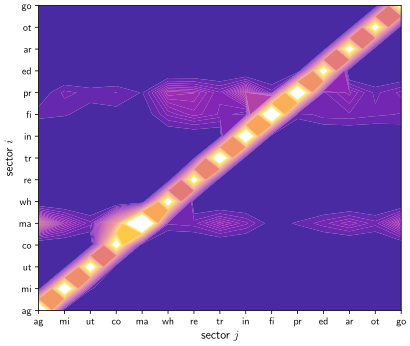
Figure 2.4:The Leontief inverse (hotter colors indicate larger values)
2.1.3.2Shock Propagation
Figure 2.5 shows the impact of a given vector of demand shocks on the 15 sector input-output model. In this simulation, each element of was drawn independently from a uniform distribution. The vector is shown visually in the panel titled “round 0,” with hotter colors indicating larger values. The shock draw was relatively large in retail (re) and information (in).
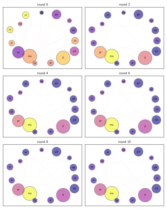
Figure 2.5:Propagation of demand shocks via backward linkages
The remaining rounds then show the values , , etc., with hotter colors indicating higher values. In each round, to make the within-round comparison between sectors clearer, values of the vector are rescaled into the interval before the color map is applied.
Note that, by round 6, the values of have settled into a fixed pattern. (This is only up to a scaling constant, since values are rescaled into as just discussed.) Manufacturing is the most active sector, while finance and professional services are also quite active. In fact, if we repeat the simulation with a new draw for , the pattern of active sectors quickly converges to exactly the same configuration.
We can explain this phenomenon using the Perron–Frobenius theorem. Since is primitive (in the 15 sector case), we know that converges to as , where and are the dominant left and right eigenvectors respectively, normalized so that . It follows that, for large , we have
In other words, up to a scaling constant, the shock response converges to the dominant right eigenvector, which is also the hub-based eigenvector centrality measure.
In Figure 2.5, the scaling constant is not visible because the values are rescaled to a fixed interval before the color map is applied. However, (2.10) shows us its value, as well as the fact that the scaling constant converges to zero like . Hence, the dominant eigenpair gives us both the configuration of the response to an arbitrary demand shock and the rate at which the response dies out as we travel back through the linkages.
At this point, we recall that the sectors in Figure 2.1 were colored according to hub-based eigenvector centrality. If you compare this figure to Figure 2.5, you will be above to confirm that, at least for later rounds, the color schemes line up, as predicted by the theory. Finance (fi) and manufacturing (ma) rank highly, as does the professional services sector (pr), which includes consulting, accounting and law.
2.1.3.3Eigenvector Centrality
Let’s look at hub-based eigenvector centrality more closely. In a production network, the hub property translates into being an important supplier. Our study of demand shocks in Section 2.1.3 highlighted the significance of the eigenvector measure of hub-based centrality: if sector has high rank under this measure, then it becomes active after a large variety of different shocks. Figure 2.6 shows hub-based eigenvector centrality as a bar graph for the 15 sector case. By this measure, manufacturing is by far the most dominant sector in the US economy.
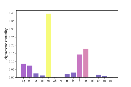
Figure 2.6:Eigenvector centrality across US industrial sectors
Reviewing the color scheme in Figure 2.2 based on our current understanding of eigenvector centrality, we see that technical servies (54120P), insurance (524), chemical products (325) and primary metals (331) are among the most highly ranked, and hence a wide range of demand shocks generate high activity in these sectors.
To provide some extra context, we show the analogous figure using Australian 2020 input-output data, collected by the Australian Bureau of Statistics. Node size is proportional to sales share and arrow width is proportional to the input-output coefficient. The color map shows hub-based eigenvector centrality.
By this measure, the highest ranked sector is 6901, which is “professional, scientific and technical services.” This includes scientific research, engineering, computer systems design, law, accountancy, advertising, market research, and management consultancy. The next highest sectors are construction and electricity generation.
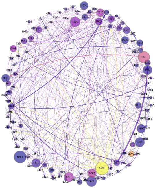
Figure 2.7:Network for 114 Australian industry sectors in 2020
2.1.3.4Output Multipliers
One way to rank sectors that has a long tradition in input-output analysis is via output multipliers. The output multiplier of sector , denoted below by , is usually defined as the “total sector-wide impact of an extra dollar of demand in sector ,” where total means taking into account backward linkages. This measure has historically been of interest to policy makers considering impacts of fiscal stimulus.
Recalling from Section 2.1.3.1 that shows the total impact on sector of a unit change in demand for good , we come to the definition
In vector notation this is or,
Comparing this with (1.39), we see that the vector of output multipliers is equal to the authority-based Katz centrality measure (with the parameter defaulting to unity).
The connection between the two measures makes sense: high authority-based centrality means that a sector has many inward links, and that those links are from other important sectors. Loosely speaking, such a sector is an important buyer of intermediate inputs. A sector highly ranked by this measure that receives a demand shock will cause a large impact on the whole production network.
Figure 2.8 shows the size of output multipiers across 15 US industrial sectors, calculated from the same input-output data as previous 15 sector figures using (2.11). The highest ranks are assigned to manufacturing, agriculture and construction.
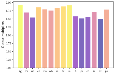
Figure 2.8:Output multipliers across 15 US industrial sectors
2.1.4Forward Linkages
Several economic questions connect to relative “upstreamness” of a sector or production good. For example, Olabisi (2020) finds that upstreamness is related to sectoral volatility, while Antràs et al. (2012) examine the relationship between upstreamness and tendency to export. Tariff changes tend to have different aggregate effects when applied to upstream rather than downstream industries Martin & Otto, 2020. Finally, since WWII, many developing countries have systematically supported and encouraged upstream industries Liu, 2019.
In order to study upstreamness, we first introduce the Ghosh model for forward linkages, which uses a rearrangement of terms from the original Leontief model.
2.1.4.1The Ghosh Model
Recall that the dollar value of inputs from per dollar of sales from . Consider now the related quantities
Let . The matrix is called the direct-output matrix or the Ghosh matrix. Element can be interpreted as the size of the “forward linkage” from to . Analogous to , the matrix can be viewed as a weight function over output sectors and visualized as in Figure 2.9. This digraph uses the same data source as Figure 2.1.
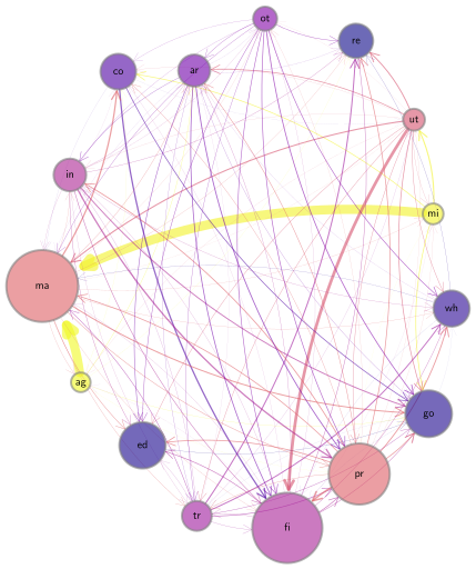
Figure 2.9:Forward linkages and upstreamness over US industrial sectors
Let be value added in sector (i.e., payments to factors of production other than intermediate goods). We have
This states that (under perfect competition), the revenue of sector is divided between spending on intermediate goods, which is the first term , and payments to other factors of production (value added).
Using the forward linkages, we can rewrite (2.13) as for all or, in matrix form
Taking transposes and solving under the assumption gives
We can think of the solution in (2.15) as the amount of output necessary to acquire a given amount of value added. Since payments of value added are made to underlying factors of production, the Ghosh model is also called a “supply-side input output model”.
We omit a discussion of the relative merits of supply- and demand-driven input-output models. Our main interest in forward linkages is due to their connection to the topic of ranking sectors by relative upstreamness.
2.1.4.2Upstreamness
Which industries are relatively upstream? One proposed measure of upstreamness can be found in Antràs et al. (2012). With as defined in (2.12), the upstreamness of sector is defined recursively by
The recursive definition of the vector in (2.16) stems from the idea that those sectors selling a large share of their output to upstream industries should be upstream themselves.
We can write (2.16) in vector form as and solve for as
A unique nonnegativity solution exists provided that . We expect this to hold in general, due to the findings in Exercise 2.1.7.
Maintaining the convention , we see that the upstreamness measure (2.17) proposed by Antràs et al. (2012) is identical to the hub-based Katz centrality measure (1.37) for the production network with weights allocated by the forward linkage matrix .
Figure 2.10 shows the result of computing via (2.17), plotted as a bar graph, for the 15 sector input-output network. Consistent with expectations, the primary commodity producers (agriculture and mining) are the most upstream, while retail and education are typical downstream sectors.
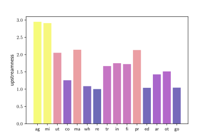
Figure 2.10:Relative upstreamness of US industrial sectors
The nodes in Figure 2.9 are also colorized by upstreamness.
2.2General Equilibrium
One limitation of the Leontief input-output analysis from Section 2.1 is that demand is fixed and exogenous. In this section we embed Leontief’s model in an equilibrium setting where output and prices are determined by a combination of supply and demand. One objective is to understand how an input-output structure interacts with firm-level shocks to shape aggregate volatility.
2.2.1Supply and Demand
Our first step is to introduce and solve a multisector general equilibrium model based on Acemoglu et al. (2012) and Carvalho & Tahbaz-Salehi (2019).
2.2.1.1Production and Prices
As in the Leontief economy, there are sectors, also called industries, each of which produces one good. Real output in sector is given by
Here
is a sector-specific shock (independent across sectors),
is labor input to sector ,
is the amount of good used in the production of good , and
and take values in and satisfy for all .
The last condition implies constant returns to scale (CRS) in each sector.[2]
Firms are price takers. With being the price of good , a firm in sector maximizes profits
with respect to the controls and .
Substituting the maximizers (2.20) into the production function gives
where is a positive constant depending only on parameters.
Let and be the column vectors and of normalized prices and log shocks from Exericse Exercise 2.2.4. Collecting the equations stated there leads to , or
As in Chapter 2, the matrix is the Leontief inverse generated by .
2.2.1.2Consumpion
Wages are paid to a representative household who chooses consumption to maximize utility . In equilibrium, profits are zero, so the only income accruing to the household consists of wage income. The household supplies one unit of labor inelastically. Hence, the budget constraint is .
2.2.1.3Aggregate Output
In this economy, aggregate value added (defined in Section 2.1.4) is equal to the wage bill. This quantity is identified with real aggregate output and referred to as GDP. The Domar weight of each sector is defined as its sales as a fraction of GDP:
From the closed economy market clearing condition and the optimality conditions we obtain
From the results of Exercise 2.2.4 we obtain . Setting and summing yields
Normalizing prices so that , this simplifies to
Thus, log GDP is the inner product of sectoral shocks and the Domar weights.
2.2.2The Granular Hypothesis
We have just constructed a multisector model of production and output. We plan to use this model to study shock propagation and aggregate fluctuations. Before doing so, however, we provide a relatively simple and network-free discussion of shock propagation. The first step is to connect the propagation of shocks to the firm size distribution. Later, in Section 2.2.3, we will see how these ideas relate to the general equilibrium model and the topology of the production network.
2.2.2.1Aggregate vs Idiosyncratic Shocks
Some fluctuations in aggregate variables such as GDP growth and the unemployment rate can be tied directly to large exogenous changes in the aggregate environment. One obvious example is the jump in the US unemployment rate from 3.5% to 14.8% between February and April 2020, which was initiated by the onset of the COVID pandemic and resulting economic shutdown.
Other significant fluctuations lack clear macro-level causes. For example, researchers offer mixed explanations for the 1990 US recession, including “technology shocks,” “consumption shocks” and loss of “confidence” Cochrane, 1994. However, these explanations are either difficult to verify on the basis of observable outcomes or require exogenous shifts in variables that should probably be treated as endogenous.
One way to account for at least some of the variability observed in output growth across most countries is on the basis of firm-level and sector-specific productivity and supply shocks. Examples of sector-specific shocks include
the spread of African Swine Fever to China in 2018,
the Great East Japan Earthquake of 2011 and resulting tsunami, which triggered meltdowns at three reactors in the Fukushima Daiichi Nuclear Power Plant, and
the destruction of Asahi Kasei Microdevices’ large scale IC factory in Miyazaki Prefecture in October 2020.
In the discussion below, we investigate the extent to which firm-level shocks can drive fluctuations in aggregate productivity.
2.2.2.2The Case of Many Small Firms
It has been argued that idiosyncratic, firm-level shocks can account only for a very small fraction of aggregate volatility (see, e.g., Dupor (1999)). The logical heart of this argument is the dampening effect of averaging over independent random variables. To illustrate the main idea, we follow a simple model of production without linkages across firms by Gabaix (2011).
Suppose there are firms, with the size of the -th firm, measured by sales, denoted by . Since all sales fulfill final demand, GDP is given by . We use primes for next period values and for first differences (e.g., ). We assume that firm growth is equal to , where is a collection of IID random variables corresponding to firm-level idiosyncratic shocks. We also assume that , so that represents firm-level growth volatility.
GDP growth is then
If, say, all firms are equal size, so that , this means that , so volatility at the aggregate level is very small when the number of firms is large. For example, if the number of firms is , which roughly matches US data, then
Hence firm-level volatility accounts for only 0.1% of aggregate volatility.
To be more concrete, Gabaix (2011) calculates , which means that, by (2.27), %. But the volatility of GDP growth is actually far higher. Indeed, Figure 2.11 reports that, for the US, is approximately , which is two orders of magnitude greater. The core message is that, under the stated assumptions, firm-level shocks explain only a tiny part of aggregate volatility.
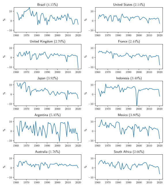
Figure 2.11:GDP growth rates and std. deviations (in parentheses) for 10 countries
2.2.2.3The Effect of Heavy Tails
There are some obvious problems with the line of reasoning used in Section 2.2.2.2. One is that firms are assumed to be of identical size. In reality, most firms are small to medium, while a relative few are enormous. For example, in the US, a small number of giants dominate technology, electronics and retail.
Gabaix (2011) emphasized that we can get closer to actual GDP volatility by more thoughtful specification of the firm size distribution. Altering the distribution changes the value in (2.27), which is called the Herfindahl index. This index is often applied to a group of firms in a sector to measure industry concentration. For given aggregate output , the Herfindahl index is minimized when for all . This is the case we considered above. The index is maximized at when a single firm dominates all sales. By (2.27), a larger Herfindahl index will increase relative to , which allows firm-level shocks to account for more of aggregate volatility.
Calculation of is challenging because the entire firm size distribution is difficult to observe. Nonetheless, we can estimate by (a) estimating a population probability distribution that fits the empirical distribution and (b) using analysis or Monte Carlo simulations to calculate typical values of .
For step (a), Gabaix (2011) cites the study of Axtell (2001), which finds the firm size distribution to be Pareto with tail index . If we repeatedly draw from a Pareto distribution with and , record the value of after each draw and then take the median value as our estimate, we obtain . In other words, under the Pareto assumption just stated, firm-level volatility accounts for almost 90% of aggregate volatility. In essence, this means that, to explain aggregate volatility, we need to look no further than firm-level shocks.
2.2.2.4Sensitivity Analysis
The finding in the previous paragraph is quite striking. How seriously should we take it?
One issue is that the figure is not robust to small changes in assumptions. For example, the regression in Figure 1.7 suggests that we take as our estimate for the tail index , rather than Axtell’s value of . If we rerun the same calculation with , the estimated value of falls to . In other words, firm-level shocks account for only 1.8% of aggregate volatility.
Another issue is that the large value for obtained under Axtell’s parameterization is very sensitive to the parametric family chosen for the firm size distribution. The next exercise illustrates.
2.2.3Network Structure and Shock Propagation
The sensitivity analysis in Section 2.2.2.4 suggests we should be skeptical of the claim that firm-level shocks explain most aggregate-level shocks that we observe. This means that either micro-level shocks account for only a small fraction of aggregate volatility or, alternatively, that the model is too simple, and micro-level shocks are amplified through some other mechanism.
An obvious way to explore further is to allow linkages between firms, in the sense that the inputs for some firms are outputs for others. Such an extension opens up the possibility that shocks propagate through the network. This seems plausible even for the sector-specific shocks listed above, such as the Great East Japan Earthquake. Although the initial impact was focused on electricity generation, the flow-on effects for other sectors were rapid and substantial Carvalho et al., 2021.
To investigate more deeply, we connect our discussion of the granular hypothesis back to the multisector models with linkages studied above, allowing us to study flow-on and multiplier effects across industries.
2.2.3.1Industry Concentration and Shocks
From (2.25) and the independence of sectoral shocks, the standard deviation of log GDP is given by
where is the standard deviation of each .
Note that the expression for aggregate volatility takes the same form as (2.26) from our discussion of the granular hypothesis in Section 2.2.2, where was called the Herfindahl index. Once again, this index is the critical determinant of how much firm-level volatility passes through to aggregate volatility. In particular, as discussed in Section 2.2.2.3, independent firm-level shocks cannot explain aggregate volatility unless is large, which in turn requires that the components of the vector are relatively concentrated in a single or small number of sectors.
To investigate an extreme case, we recall from Exercise 2.2.8 that . The Herfindahl index is , where is the Euclidean norm.
Under this configuration of sector shares,
Hence, by (2.28), we have . This is the classic diversification result. The standard deviation of log GDP goes to zero like , as in the identical firm size case in Section 2.2.2.2.
Now let’s consider the other extreme:
This is the extreme case of zero diversification. By (2.25), log GDP is then
The volatility of log GDP is constant in , rather than declining in the number of sectors. In other words, idiosyncratic and aggregate shocks are identical.
2.2.3.2The Role of Network Topology
In the previous section we looked at two extreme cases, neither of which is realistic. Now we look at intermediate cases. In doing so, we note an interesting new feature: unlike the analysis in Section 2.2.2, where the sector shares were chosen from some fixed distribution, the Herfindahl index is now determined by the network structure of production.
To see this, we can use the results of Exercise 2.2.7 to obtain
Recalling our discussion in Section 1.4.3.5, we see that the vector of Domar weights is just a rescaling of the vector of hub-based Katz centrality rankings for the input-output matrix. Thus, the propagation of sector-specific productivity shocks up to the aggregate level depends on the distribution of Katz centrality across sectors. The more “unequal” is this distribution, the larger is the pass through.
Figure 2.13 shows some examples of different network configurations, each of which is associated with a different Katz centrality vector. Not surprisingly, the symmetric network has a constant centrality vector, so that all sectors have equal centrality. This is the maximum diversification case, as discussed in Section 2.2.3.1. The other two cases have nonconstant centrality vectors and hence greater aggregate volatility.[5]
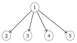
Figure 2.12:Star network with single hub
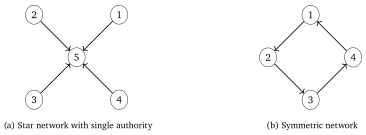
Figure 2.13:Symmetric and asymmetric networks
The results of Exercise 2.2.13 show that the hub network has the more unequal Katz centrality vector. Not surprisingly, the source node in the hub has a high hub-based centrality ranking. Productivity shocks affecting this sector have a large effect on aggregate GDP.
Figure 2.14 shows hub-based Katz centrality computed from the 15 sector input-output data for 2021. We can see that productivity shocks in manufacturing will have a significantly larger impact on aggregate output than shocks in say, retail or education.
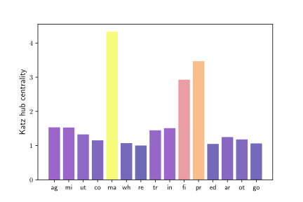
Figure 2.14:Hub-based Katz centrality of across 15 US industrial sectors
2.2.3.3Supply Shocks vs Demand Shocks
In the previous section we saw that the degree to which a productivity shock propagates through the economy depends on the hub-based centrality ranking of the relevant sector. This is intuitive. Sectors that act like hubs supply many sectors, so changes in productivity in these sectors will have large flow-on effects.
This is in contrast with what we learned in Section 2.1.3.4, where a high authority-based centrality measure lead to high shock propagation. The difference can be explained by the source of the shocks: in Section 2.1.3.4, we were concerned with the impact of demand shocks. Demand shocks to sector have large flow-on effects when many sectors purchase inputs from sector . Hence authority-based centrality measures are appropriate for studying this case.
2.3More Spectral Theory
This is a relatively technical section, which analyzes aspects of vector dynamics and spectral theory in more depth. It is aimed at readers who are interested in further mathematical discussion of the theory treated above. The ideas studied here are applied to production problems to generate additional insights into existence and uniqueness of equilibria, as well as later topics such as convergence of distributions for Markov models on networks.
2.3.1Vector Norms
In this section we learn about abstract vector norms on and provide several examples. Later we will see how the different norms are related and how they can be useful for some kinds of network analysis.
2.3.1.1Norms
A function is called a norm on if, for any and ,
and
(nonnegativity)
(positive definiteness)
(positive homogeneity)
(triangle inequality)
The Euclidean norm is a norm on , as suggested by its name.
The norm and the Euclidean norm are special cases of the so-called norm, which is defined for by
It can be shown that is a norm for all , as suggested by the name (see, e.g., Kreyszig (1978)). For this norm, the subadditivity in (d) is called Minkowski’s inequality.
Since the Euclidean case is obtained by setting , the Euclidean norm is also called the norm, and we write rather than when extra clarity is required.
(The symbol is used because, , we have as .) This norm is called the supremum norm.
2.3.1.2Equivalence of Vector Norms
When and are all elements of , we say that converges to and write if
It might seem that this definition is imprecise. Don’t we need to clarify that the convergence is with respect to a particular norm?
In fact we do not. This is because any two norms and on are equivalent, in the sense that there exist finite constants such that
Another way to understand is via pointwise convergence: each element of the vector sequence converges to the corresponding element of . Pointwise and norm convergence are equivalent, as the next result makes clear.
2.3.2Matrix Norms
In some applications, the number of vertices of a given digraph is measured in millions or billions. This means that the adjacency matrix is enormous. To control complexity, must often be replaced by a sparse approximation . It is natural to require that and are close. But how should we define this?
More generally, how can we impose a metric on the set of matrices to determine similarity or distance between them? One option is to follow the example of vectors on and introduce a norm on . With such a norm in hand, we can regard and as close when is small.
For this and other reasons, we now introduce the notion of a matrix norm.
2.3.2.1Definition
Analogous to vectors on , we will call a function from to a norm if for any ,
and
(nonnegativity)
(positive definiteness)
(positive homogeneity)
(triangle inequality)
The distance between two matrices is then specified as .
Unlike vectors, matrices have a product operation defined over all conformable matrix pairs. We want matrix norms to interact with this product in a predictable way. For example, it is helpful for analysis when a matrix norm is submultiplicative, meaning that
A useful implication of (2.32) is that for any and , where is the -th power of .
2.3.2.2The Frobenius Norm
One way to construct a norm on matrix space is to first introduce the Frobenius inner product of matrices as
From this inner product, the Frobenius norm of is defined as
In essence, the Frobenius norm converts an matrix into an vector and computes the Euclidean norm.
The Frobenius norm is submultiplicative. The next exercise asks you to prove this in one special case.
2.3.2.3The Operator Norm
Another important matrix norm is the operator norm, defined at by
where the norm on the right hand size of (2.35) is the Euclidean norm on .
2.3.2.4Other Matrix Norms
Two other useful matrix norms are the and norms given by
2.3.2.5Equivalence of Matrix Norms
In Section 2.3.1.2 we saw that all norms on are equivalent. Exactly the same result holds true for matrix norms: any two norms and on are equivalent, in the sense that there exist finite constants such that
A proof can be found (for abstract finite-dimensional vector space) in Bollobás (1999).
Analogous to the vector case, given and in , we say that converges to and write if as , where is a matrix norm. Once again, we do not need to clarify the norm due to the equivalence property. Also, norm convergence is equivalent to pointwise convergence:
2.3.3Iteration in Matrix Space
Results such as Proposition 1.4.2 already showed us the significance of powers of adjacency matrices. The Perron-Frobenius theorem revealed connections between spectral radii, dominant eigenvectors and powers of positive matrices. In this section we investigate powers of matrices in more depth.
2.3.3.1Gelfand’s Formula
One very general connection between matrix powers and spectral radii is Gelfand’s formula for the spectral radius:
Proofs can be found in Bollobás (1999) or Kreyszig (1978).
The next exercise shows that implies at a geometric rate.
2.3.3.2A Local Spectral Radius Theorem
The next theorem is a “local” version of Gelfand’s formula that relies on positivity. It replaces matrix norms with vector norms, which are easier to compute.
Theorem 2.3.3 tells us that, eventually, for any positive , the norm of the vector grows at rate . A proof can be found in Krasnoselskii (1964).[6]
2.3.3.3Convergence to the Perron Projection
The local spectral radius theorem assumes . Now we further strengthen this assumption by requiring that is primitive. In this case, converges to the Perron projection as (see (1.11)). We want rates of convergence in high-dimensional settings.
We fix and label the eigenvalues so that for all . Note that . Let be the Perron projection.
Thus, an upper bound on the rate of convergence to the Perron projection is determined by the modulus of the ratio of the first two eigenvalues.
2.3.4Exact Stability Conditions
The Neumann series lemma tells us that the linear system has a unique solution whenever . We also saw that, in the input-output model, where is the adjacency matrix, the condition holds whenever every sector has positive value added (Assumption 2.1.1 and Exercise 2.1.2). Hence we have sufficient conditions for stability.
This analysis, while important, leaves open the question of how tight the conditions are and what happens when they fail. For example, we might ask
To obtain , is it necessary that each sector has positive value added? Or can we obtain the same result under weaker conditions?
What happens when fails? Do we always lose existence of a solution, or uniqueness, or both?
In Section 2.3.4.1 and Section 2.3.4.2 below we address these two questions.
2.3.4.1Spectral Radii of Substochastic Matrices
To reiterate, the results in Section 5.1.3 relied on the assumption that every sector has positive value added, which in turn gave us the property for the adjacency matrix of the input-output production network. Positive value added in every sector is not necessary, however. Here we investigate a weaker condition that is exactly necessary and sufficient for . This weaker condition is very helpful for understanding other kinds of networks too, including financial networks, as discussed in Section 5.2.
To begin, recall that a matrix is called stochastic if and . Similarly, is called substochastic if and . Thus, a substochastic matrix is a nonnegative matrix with less than unit row sums. Clearly the transpose of a nonnegative matrix is substochastic if and only if has less than unit column sums.
A natural example of a substochastic matrix is the transpose of an adjacency matrix of an input-output network. Indeed, such an is nonnegative and, for -th column sum we have
Hence , which says that spending on intermediate goods and services by a given industry does not exceed total sales revenue, is a necessary condition for nonnegative profits in sector . When this holds for all , the adjacency matrix has less than unit column sums.
From Lemma 1.2.7, we see that any substochastic matrix has
We wish to know when we can tighten this to .
From (2.41), one obvious sufficient condition is that for all . This is, in essence, how we used Assumption 2.1.1 (every sector has positive value added) in the input-output model. Under that condition we have for all , which says all column sums are strictly less than one. Hence
where the middle implication is by (2.41) and the last equivalence is by .
Now we provide a weaker—in fact necessary and sufficient—condition for , based on network structure. To do so, we define an substochastic matrix to be weakly chained substochastic if, for all , there exists an such that and . Here accessibility of from is in terms of the induced weighted digraph.[7]
A proof can be found in Corollary 2.6 of Azimzadeh (2019).
Now we return to the input output model. Let’s agree to say that sector is an upstream supplier to sector if in the input-output network. By Proposition 1.4.2, an equivalent statement is that there exists a such that .
2.3.4.2A Converse to the Neumann Series Lemma
Since the Neumann series lemma is a foundational result with many economic applications, we want to know what happens when the conditions of the lemma fail. Here is a partial converse:
2.4Chapter Notes
High quality foundational textbooks on input-output analysis and multisector production networks include Nikaido (1968), Miller & Blair (2009) and Antras (2020). References on production networks and aggregate shocks include Acemoglu et al. (2012), Antràs et al. (2012), Di Giovanni et al. (2014), Carvalho (2014), Barrot & Sauvagnat (2016), Baqaee (2018), Carvalho & Tahbaz-Salehi (2019), Acemoglu & Azar (2020), Liu & Tsyvinski (2020), Miranda-Pinto (2021) and Carvalho et al. (2021).
For other network-centric analysis of multisector models, see, for example, Bernard et al. (2019), who use buyer-supplier relationship data from Belgium to investigate the origins of firm size heterogeneity when firms are interconnected in a production network. Herskovic (2018) analyzes asset pricing implications of production networks. Cai & Szeidl (2018) consider the effect of interfirm relationships on business performance. La'O & Tahbaz-Salehi (2022) study optimal monetary policy in a production network. Dew-Becker (2022) analyzes tail risk and aggregate fluctuations in a nonlinear production network. Elliott et al. (2022) show that complex supply networks can greatly amplify small idiosyncratic shocks. Elliott & Golub (2022) provide a survey of network fragility that includes discussion of production networks and the impact of sectoral shocks.
We obtain input expenditures and total sales for each sector from the Make-Use Tables of the Input-Output Accounts Data. The figure was created using Python’s Networkx library.
In order to be consistent with traditional input-output notation (see Section 2.1), we transpose and relative to sources such as Acemoglu et al. (2012) and Carvalho & Tahbaz-Salehi (2019). This is just a matter of convention.
Later, in Section 2.3, we use additional spectral theory to prove the exact result .
In other words, each is an independent copy of the random variable , where is standard normal.
The captions in Figure 2.13 refer to these two cases as “star networks,” in line with recent usage in multisector production models. In graph theory, a star network is an undirected graph that (a) is strongly connected and (b) has only one node with degree greater than one.
A direct proof of a generalized version of Theorem 2.3.3 is provided in Theorem B1 of Borovička & Stachurski (2020).
Induced weighted digraphs are defined in Section 1.4.2.1. By Proposition 1.4.2, accessibility of from is equivalent to existence of a with , where is the -th element of (and ).
- Leontief, W. W. (1941). The Structure of American Economy, 1919-1929. Harvard University Press.
- Olabisi, M. (2020). Input–Output Linkages and Sectoral Volatility. Economica, 87(347), 713–746.
- Antràs, P., Chor, D., Fally, T., & Hillberry, R. (2012). Measuring the upstreamness of production and trade flows. American Economic Review, 102(3), 412–416.
- Martin, T., & Otto, C. A. (2020). The Downstream Impact of Upstream Tariffs: Evidence from Investment Decisions in Supply Chains [Techreport]. SSRN 2872662.
- Liu, E. (2019). Industrial policies in production networks. The Quarterly Journal of Economics, 134(4), 1883–1948.
- Acemoglu, D., Carvalho, V. M., Ozdaglar, A., & Tahbaz-Salehi, A. (2012). The network origins of aggregate fluctuations. Econometrica, 80(5), 1977–2016.
- Carvalho, V. M., & Tahbaz-Salehi, A. (2019). Production networks: A primer. Annual Review of Economics, 11, 635–663.
- Cochrane, J. H. (1994). Shocks. Carnegie-Rochester Conference Series on Public Policy, 41, 295–364.
- Dupor, B. (1999). Aggregation and irrelevance in multi-sector models. Journal of Monetary Economics, 43(2), 391–409.
- Gabaix, X. (2011). The granular origins of aggregate fluctuations. Econometrica, 79(3), 733–772.
- Axtell, R. L. (2001). Zipf distribution of US firm sizes. Science, 293(5536), 1818–1820.
- Kondo, I. O., Lewis, L. T., & Stella, A. (2020). Heavy Tailed, but not Zipf: Firm and Establishment Size in the US [Techreport]. Federal Reserve Bank of Minneapolis.
- Carvalho, V. M., Nirei, M., Saito, Y. U., & Tahbaz-Salehi, A. (2021). Supply chain disruptions: Evidence from the great east japan earthquake. The Quarterly Journal of Economics, 136(2), 1255–1321.
- Kreyszig, E. (1978). Introductory functional analysis with applications (Vol. 1). wiley New York.
- Bollobás, B. (1999). Linear Analysis: An Introductory Course. Cambridge University Press.