Markov chains evolving on finite sets are a foundational class of stochastic processes. These processes have been employed in quantitative economics to study stochastic systems ranging from labor income to harvest outputs, firm productivity, stock prices, unemployment dynamics, policy regimes, interest rates, and social mobility. Fortunately, we are now well placed to study Markov chains, since such chains are most naturally viewed as a special kind of weighted digraph. Moreover, graph-theoretic properties such as connectedness and periodicity are key determinants of their dynamics. In this chapter we investigate these ideas.
4.1Markov Chains as Digraphs
We begin with fundamental definitions and then investigate dynamics.
4.1.1Markov Models
A finite Markov model is a weighted directed graph , where is the (finite) set of vertices, is the set of edges and is the weight function, with the additional restriction that
Figure 1.15 presented an example of such a digraph.
The set of vertices of a finite Markov model is also called the state space of the model, and vertices are called states. The two standard interpretations are
is a set of possible states for some random element (the state) and the weight represents the probability that the state moves from to in one step.
is a set of possible values for some measurement over a large population (e.g., hours worked per week measured across a large cross-section of households) and is the fraction of agents that transition from state to state in one unit of time.
These two perspectives are related in ways that we explore below.
4.1.1.1Transition Matrices
If is a finite Markov model, then the restriction (4.1) is equivalent to the statement that the adjacency matrix associated with is stochastic (see Section 1.3.1.3 for the definition). Identifying with , the adjacency matrix for this weighted digraph is
Since and rows sum to unity, is stochastic as required. In the context of finite Markov models, the adjacency matrix of is also called the transition matrix.
Regarding notation, when has typical elements , it turns out to be convenient to write elements of the transition matrix as rather than or similar. We can think of as extending the weight function from to the set of all pairs in , assigning zero whenever . As such, for every possible choice of , the value represents the probability of transitioning from to in one step.
The requirement that is stochastic can now be written as and
The restriction in (4.3) just says that the state space is “complete:” after arriving at , the state must now move to some .
Using notation from Section 1.3.1, to say that is stochastic is the same as requiring that each row of is in .
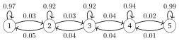
Figure 4.1:Cross-country GDP dynamics as a digraph
The transition matrix for the Markov model in Example 4.1.1 is
Note the large values on the principal diagonal of . These indicate strong persistence: the state stays constant from period to period with high probability.
Quah (1993) estimated by maximum likelihood, pooling transitions over the years 1960–1984. (In this case maximum likelihood estimation amounts to recording the relative frequency of transitions between states.) Figure 4.2 shows how the numbers change if we repeat the exercise using World Bank GDP data from 1985–2019. The numbers are quite stable relative to the earlier estimate. Below we will examine how long run predictions are affected.
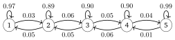
Figure 4.2:Cross-country GDP dynamics as a digraph, updated data
As another example, Benhabib et al. (2019) estimate the following transition matrix for intergenerational social mobility:
Here the states are percentiles of the wealth distribution. In particular, with the states represented by , the corresponding percentiles are
0–20%, 20–40%, 40–60%, 60–80%, 80–90%, 90–95%, 95–99%, 99–100%
Transition probabilities are estimated from US 2007–2009 Survey of Consumer Finances data. Relative to the highly persistent matrix , less weight on the principle diagonal suggests more mixing—the influence of initial conditions is relatively short-lived.
Additional insight about the dynamics can be obtained from a contour plot of the matrix , as in Figure 4.3. Here is plotted as a heat map after rotating it 90 degrees anticlockwise. The rotation is so that the dynamics are comparable to the 45 degree diagrams often used to understand discrete time dynamic systems. A vertical line from state corresponds to the next period conditional distribution .
In this case, we see that, for example, lower states are quite persistent, whereas households in the highest state tend to fall back towards the middle.
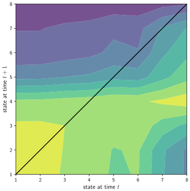
Figure 4.3:Contour plot of transition matrix
4.1.1.2Markov Chains
Consider a finite Markov model with state space and transition matrix . As before, indicates the probability of transitioning from to in one step. Another way to say this is that, when in state , we update to a new state by choosing it from via the distribution . The resulting stochastic process is called a Markov chain.
We can state this more formally as follows. Let be a sequence of random variables taking values in . We say that is a Markov chain on if there exists a stochastic matrix on such that
To simplify terminology, we also call -Markov when it satisfies (4.7) . We call either or its distribution the initial condition of depending on context.
The definition of a Markov chain says two things:
When updating to from , earlier states are not required.
The matrix encodes all of the information required to perform the update, given .
One way to think about Markov chains is algorithmically: Let be a stochastic matrix and let be an element of . Now generate via Algorithm 3. The resulting sequence is -Markov with initial condition .
4.1.1.3Simulation
For both simulation and theory, it is useful to be able to translate Algorithm 3 into a stochastic difference equation governing the evolution of . We now outline the procedure, which uses inverse transform sampling (see Section 1.3.1.2). For simplicity, we assume that , with typical elements . The basic idea is to apply the inverse transform method to each row of and then sample by drawing a uniform random variable at each update.
To this end, we set
where, for each , the value is defined recursively by
Let represent the uniform distribution on and take
If is an independently drawn random variable with distribution on , then is -Markov on with initial condition , as Exercise 4.1.2 asks you to show.
Each subfigure in Figure 4.4 shows realizations of two Markov chains, both generated using the stochastic difference equation (4.8). The sequences are generated each with its own independent sequence of draws . The underlying transition matrices are from (4.5) in the top panel and from (4.4) in the bottom panel. In both panels, one chain starts from the lowest state and the other from the highest. Notice that time series generated by mix faster than those generated by : the difference in initial states is not a strong predictor of outcomes after an initial “burn in” period. We discuss mixing and its connection to stability below.
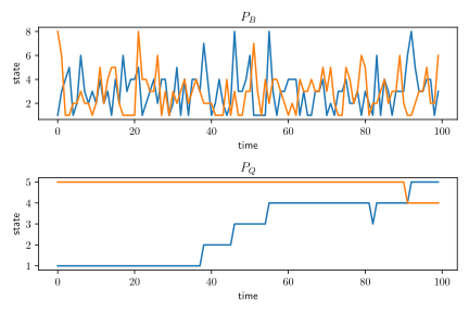
Figure 4.4:Wealth percentile over time
4.1.1.4Higher Order Transition Matrices
Given a finite Markov model with state space and transition matrix , define by for all , with the understanding that the identity matrix. In other words, for each , the matrix is the -th power of . If we spell out the matrix product element-by-element, we get
In this context, is called the -step transition matrix corresponding to . The -step transition matrix has the following interpretation: If is -Markov, then, for any and ,
In other words, provides the -step transition probabilities for the -Markov chain , as suggested by its name.
This claim can be verified by induction. Fix and . The claim is true by definition when . Suppose the claim is also true at and now consider the case . By the law of total probability, we have
The induction hypothesis allows us to use (4.10), so the last equation becomes
This completes our proof by induction.
A useful identity for the higher order Markov matrices is
which holds for any in . This is called the Chapman–Kolmogorov equation. Note that
To provide probabilistic intuition for the validity of the Chapman–Kolmogorov equation, let and let be given. Using the law of total probability again, we have
By Markov property (4.7), the future and past are independent given the present, so
As a result of this fact and (4.10), the equation before this one can be rewritten as (4.11).
4.1.2Distribution Dynamics
Let be a finite Markov model with state space and transition matrix . Let be -Markov and, for each , let be defined by
The vector is called the marginal distribution of . While is random, the sequence is deterministic. In this section we investigate its dynamics.
4.1.2.1Updating Marginal Distributions
The key idea for this section is that there is a simple link between successive marginal distributions: by the law of total probability, we have
which can be rewritten as
This fundamental expression tells how to update marginal distributions given the transition matrix .
When each is interpreted as a row vector, we can write (4.12) as
(Henceforth, in expressions involving matrix algebra, distributions are row vectors unless otherwise stated). Some authors refer to (4.13) as the forward equation associated with , while is called the forward operator, by analogy with the Kolmogorov forward equation from continuous time.
Think of (4.13) as a difference equation in distribution space. Iterating backwards,
Given any and , we have
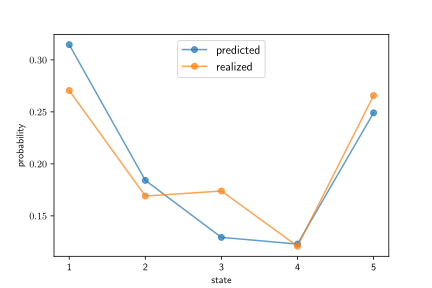
Figure 4.5:Predicted vs realized cross-country income distributions for 2019
4.1.2.2Trajectories in the Long Run
One of the main sub-fields of Markov chain analysis is asymptotics of distribution sequences. This topic turns out to be important for network theory as well. In Section 4.2.2 we will investigate asymptotics in depth. In this section we build some intuition via simulations.
Figure 4.6 shows the trajectory when , , and is the transition matrix displayed in (4.2). The blue triangle is the unit simplex in , consisting of all row vectors such that and . The unit simplex can be identified with when . Red dots in the figure are distributions in the sequence for . Figure 4.7 shows distribution dynamics for that start from initial condition .
It seems that both of the sequences are converging. This turns out to be the case—the black dot in the figures is the limit of both sequences and, moreover, this point is a stationary distribution for , as defined in Section 1.3.1.3. In fact we can—and will—also show that no other stationary distribution exists, and that converges to the stationary distribution regardless of the choice of . This is due to certain properties of , related to connectivity and aperiodicity.
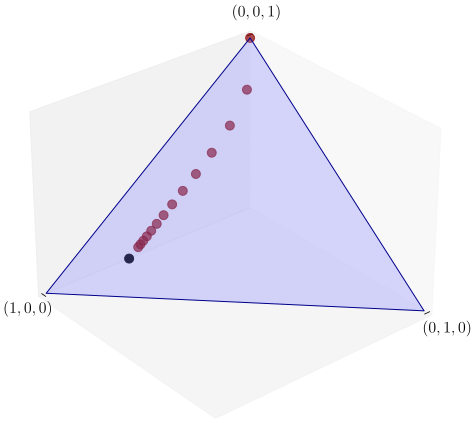
Figure 4.6:A trajectory from
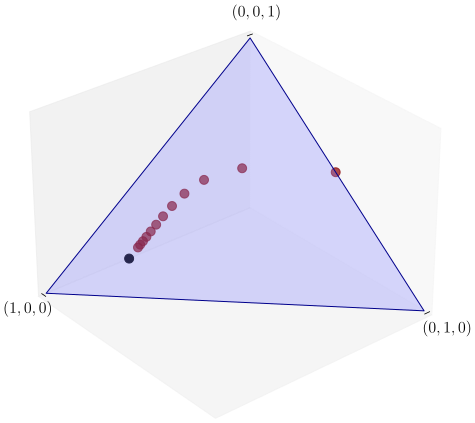
Figure 4.7:A trajectory from
Figure 4.8 provides another view of a distribution sequence, this time generated from the matrix in (4.5). The initial condition was uniform. Each distribution shown was calculated as for different values of . The distribution across wealth classes converges rapidly to what appears to be a long run limit. Below we confirm that this is so, and that the limit is independent of the initial condition. The rapid rate of convergence is due to the high level of mixing in the transition dynamics.
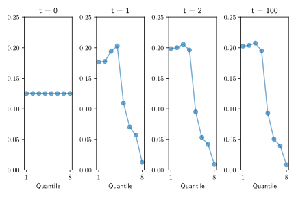
Figure 4.8:Distribution projections from
4.1.3Stationarity
In this section we examine stationary distributions and their properties. As we will see, stationary distributions can be regarded as steady states for the evolution of the sequence of marginal distributions. (Later, when we study ergodicity, stationary distributions will acquire another important interpretation.)
4.1.3.1Stationary Distributions
Recall from Section 1.3.1.3 that if is a stochastic matrix and is a row vector such that and , then is called stationary for . So now let be a finite Markov model with state space and transition matrix . Translating to the notation of Markov chains, a distribution is stationary for if
We also write this expression as and understand as a fixed point of the map that updates distributions (cf., Equation (4.13)).
If , then, for any , the fixed point property implies that . Hence
In Figure 4.6–Figure 4.7 all trajectories converge towards the stationary distribution. Not all stationary distributions have this “attractor” property, and in general there can be many stationary distributions. The next example illustrates.
4.1.3.2Existence and Uniqueness
From the Perron–Frobenius Theorem we easily obtain the following fundamental result.
The basic idea behind the uniqueness part of Theorem 4.1.1 is as follows: Suppose to the contrary that is strongly connected and yet two distinct stationary distributions and exist in . Since a -Markov chain started at always has marginal distribution and likewise for , different initial conditions lead to different long run outcomes. This contradicts strong connectedness in the following way: strong connectedness implies that both chains traverse the whole state space. Moreover, being Markov chains, they forget the past once they arrive at any state, so the starting draws should eventually be irrelevant.
(Actually, the story in the last paragraph is incomplete. Initial conditions can determine long run outcomes under strong connectedness in one sense: a “periodic” Markov model can traverse the whole space but only at specific times that depend on the starting location. If we rule out such periodicity, we get results that are even stronger than Theorem 4.1.1. This topic is treated in Section 4.2.2.)
4.1.3.3Brouwer’s Theorem
Another way to prove the existence claim in Theorem 4.1.1 is via the famous fixed point theorem of L. E. J. Brouwer (1881–1966).
The proof of Theorem 4.1.2 in one dimension is not difficult, while the proof in higher dimensions is challenging. See, for example, Aliprantis & Border (1999).
One advantage of Brouwer’s fixed point theorem is that its conditions are quite weak. One disadvantage is that it provides only existence, without uniqueness or stability. Figure 6.4 provides an example of how multiple fixed points can coexist under the conditions of the theorem.[2]
4.1.3.4Computation
Let’s consider how to compute stationary distributions. While is a finite set of linear equations that we might hope to solve directly for , there are problems with this idea. For example, is a solution that fails to lie in .
To restrict the solution to we proceed as follows: Suppose and note that row vector is stationary if and only if , where is the identity matrix. Let be the row vector . Let be the matrix of ones.
Solving the linear system (4.15) produces a stationary distribution in any setting where the stationary distribution is unique. When this is not the case, problems can arise.
There are also graph-theoretic algorithms for computing all of the stationary distributions of an arbitrary stochastic matrix. (The Python and Julia libraries QuantEcon.py and QuantEcon.jl have efficient implementations of this type.)
4.2Asymptotics
In this section we turn to long run properties of Markov chains, including ergodicity. With these ideas in hand, we will then investigate the evolution of information over social networks.
4.2.1Ergodicity
Let’s begin with the fascinating and important topic of ergodicity. The simplest way to understand ergodicity is as an extension of the law of large numbers from IID sequences to more general settings, where the IID property holds only in a limiting sense.
4.2.1.1Harmonic Functions
Let be a finite Markov model with state space and transition matrix . Fix and let
If is understood as a column vector in , then is just element of the vector . The map is sometimes called the “conditional expectation operator,” since, given that , we have
A function is called -harmonic if pointwise on . Thus, -harmonic functions are fixed points of the conditional expectation operator .
If is -harmonic and is -Markov, then
(A stochastic process with this property—i.e., that the current value is the best predictor of next period’s value—is called a martingale. Martingales are one of the foundational concepts in probability, statistics and finance.)
4.2.1.2Definition and Implications
Let be a finite Markov model with state space and transition matrix . We know that every constant function in is -harmonic. We call ergodic if the only -harmonic functions in are the constant functions.
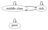
Figure 4.9:A poverty trap
The examples discussed above suggest that, for a finite Markov model , ergodicity depends on the connectivity properties of the digraph. The next result confirms this.
The implication in Proposition 4.2.1 is one way, as the next exercise asks you to confirm.
4.2.1.3Implications of Ergodicity
One of the most important results in probability theory is the law of large numbers (LLN). In the finite state setting, the classical version of this theorem states that
when is an IID sequence of random variables with common distribution and is an arbitrary element of .
This version of the LLN is classical in the sense that the IID assumption is imposed. It turns out that the IID assumption can be weakened to allow for a degree of dependence between observations, which leads us to ask whether or not the LLN holds for Markov chains as well.
The answer to this question is yes, provided that dependence between observations dies out fast enough. One candidate for this condition is ergodicity. In fact, it turns out that ergodicity is the exact necessary and sufficient condition required to extend the law of large numbers to Markov chains. The next theorem gives details.
The proof of Theorem 4.2.2 is given in Chapter 17 of Meyn & Tweedie (2009). We skip the proof but provide intuition through the following examples.
4.2.1.4Reinterpreting the Stationary Distribution
Ergodicity has many useful implications. One is a new interpretation for the stationary distribution. To illustrate this, let be an ergodic Markov model with state space and transition matrix . Let be a -chain and let
The value measures the fraction of time that the -chain spends in state over the time interval . Under ergodicity, for fixed , we can use (4.18) with to obtain
Turning (4.19) around, we see that
Figure 4.10 illustrates this idea for a simulated Markov chain generated from the matrix introduced in (4.5). The figure compares and for different values of . As , the convergence claimed in (4.19) occurs.
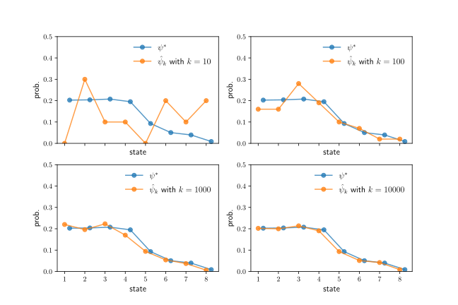
Figure 4.10:Convergence of the empirical distribution to
Of course, we must remember that (4.20) is only valid under ergodicity. For example, if , the identity, then every distribution is stationary, every -Markov chain is constant, and (4.20) does not hold.
Notice that, in view of Theorem 4.2.2, the convergence in (4.18) occurs for any initial condition. This gives us, under ergodicity, a way of computing the stationary distribution via simulation (and (4.19)). While this method is slower than algebraic techniques (see, e.g., Section 4.1.3.4) for small problems, it can be the only feasible option when is large.
4.2.2Aperiodicity and Stability
In Section 4.2.1 we discussed sample path properties of Markov chains, finding that strong connectivity is sufficient for stability of time series averages. Next we turn to marginal distributions of the chain and their long run properties, which we examined informally in Section 4.1.2.2. We will see that, to guarantee convergence of these sequences, we also need a condition that governs periodicity.
4.2.2.1Convergence of Marginals
Let be a finite Markov model with state space and transition matrix . We call globally stable if there is only one stationary distribution in and, moreover,
In other words, marginal distributions of every -Markov chain converge to the unique stationary distribution of the model.
There is a useful connection between global stability and absorbing sets. Intuitively, if is globally stable and has an absorbing set that can be reached from any , then any Markov chain generated by these dynamics will eventually arrive in and never leave. Hence the stationary distribution must put all of its mass on . The next exercise asks you to confirm this.
4.2.2.2A Key Theorem
From Theorem 4.1.1 we saw that strong connectedness is sufficient for uniqueness of the stationary distribution. One might hope that strong connectedness is enough for global stability too, but this is not true. To see why, suppose for example that and . The transition matrix is
While this model is strongly connected, global stability fails. Indeed, if is -Markov and starts at , then will visit state 1 on odd dates and state 0 on even dates. That is, . This sequence does not converge.
The issue with is that, even though the chain traverses the whole state space, the distribution of will affect that of for all due to periodicity. This causes stability to fail. If, however, we rule out periodicity, then we have enough for stability to hold. This line of reasoning leads to the following famous theorem.
The aperiodicity condition in Theorem 4.2.3 is, in general, not stringent. On the other hand, the strong connectedness requirement is arguably quite strict. Weaker conditions for global stability are available, as we shall see in Section 4.2.3.
4.2.2.3Rates of Convergence: Spectral Gap
While global stability is a very useful property, the implications are qualitative rather than quantitative. In practice, we usually want to know something about the rate of convergence. There are several ways of looking at this. We cover the two most common in this section and the next.
As a first step, fixing a Markov model with state space and transition matrix , we use (1.5) to write as
where each is an eigenvalue of and and are the right and left eigenvectors corresponding to . We have also ordered the eigenvalues from smallest to largest, and used the Perron–Frobenius Theorem to infer that , as well as the arguments in the proof of Theorem 4.2.3 that showed and .
Premultiplying by arbitrary and rearranging now gives
Recall that eigenvalues are ordered from smallest to largest and. Moreover, by the Perron–Frobenius Theorem, for all when is primitive (i.e., is strongly connected and aperiodic). Hence, after taking the Euclidean norm deviation, we obtain
Thus, the rate of convergence is governed by the modulus of the second largest eigenvalue.
The difference between the largest and second largest eigenvalue of a nonnegative matrix is often called the spectral gap. For this reason, we can also say that, for primitive stochastic matrices, the rate of convergence is determined by the (nonzero) spectral gap.
4.2.3The Markov–Dobrushin Coefficient
The rate of convergence of to given in Section 4.2.2.3 restricts the Euclidean distance between these vectors as a function of . There are, however, other metrics we could use in studying rates of convergence, and sometimes these other metrics give more convenient results. In fact, as we show in this section, a good choice of metric leads us to a more general stability result than the (better known) aperiodicity-based result in Section 4.2.2.
4.2.3.1An Alternative Metric
For the purposes of this section, For , we set
which is just the deviation between and (see Section 2.3.1.1).
Property (ii) is called the nonexpansiveness property of stochastic matrices under the deviation. As we will see, we can tighten this bound when satisfies certain properties.
As a first step we note that, for the deviation, given any stochastic matrix , we have
where
Here when . We call the Markov–Dobrushin coefficient of , although other names are also used in the literature. A proof of the bound in (4.27) can be found in Stachurski (2022) or Seneta (2006).[3]
How should the Markov–Dobrushin coefficient be understood? The coefficient is large when the rows of are relatively similar. For example, if rows and are identical, the . Similarity of rows is related to stability. The next exercise helps to illustrate.
Since powers of stochastic matrices are again stochastic, and since (4.27) is valid for any stochastic matrix, the bound in (4.29) can be generalized by replacing with for any given , which gives (with replaced by )
Now observe that, for any , we can write , where and . Fixing and choosing to make this equality hold, we get
where the second inequality is due to the nonexpansive property of stochastic matrices (Exercise 4.2.4). Since is an integer satisfying , where is the floor function, we can now state the following.
To see why the global stability implication stated in Theorem 4.2.4 holds, suppose there exists a such that . Now substitute arbitrary and any stationary distribution for into (4.30) to obtain
for all , where the second bound is due to Exercise 4.2.4.
One of the major advantages of Theorem 4.2.4 is that strong connectivity of is not required. In the next section we will see an example of a finite Markov model where (i) strong connectivity fails but (ii) the conditions of Theorem 4.2.4 are satisfied.[4]
4.2.3.2Sufficient Conditions
While the Markov–Dobrushin coefficient can be calculated for any given on a computer by stepping through all pairs of rows in , this calculation is computationally intensive when is large. When applicable, the following lemma simplifies the problem by providing a sufficient condition for .
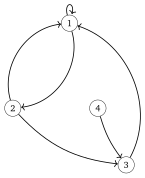
Figure 4.11:A digraph with walk of length 2 from any node to 1
4.2.3.3Application: PageRank
In Section 1.4.3 we discussed centrality measures for networks. Centrality measures provide a ranking of vertices in the network according to their “centrality” or “importance.” One of the most important applications of ranking of vertices in a network is ranking the importance of web pages on the internet. Historically, the most prominent example of a ranking mechanism for the internet is PageRank, which transformed Google from a minor start up to a technology behemoth. In this section we provide a simple introduction to the original form of PageRank and connect it to previously discussed measures of centrality.
Consider a finite collection of web pages and let be the hyperlinks between them. We understand as a digraph , where is the vertices and is the edges. Let be the associated adjacency matrix, so that if there is a link from to and zero otherwise. We set , so that is .
To start our analysis, we consider the case where is strongly connected, such as the small network in Figure 4.12. Furthermore, we introduce a second matrix in which each row of has been normalized so that it sums to one. For the network in Figure 4.12, this means that
Now consider an internet surfer who, once per minute, randomly clicks on one of the outgoing links on a page, each link selected with uniform probability . The idea of PageRank is to assign to each page a value equal to the fraction of time that this surfer spends on page over the long run. Intuitively, a high value for indicates a heavily visited and hence important site.
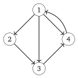
Figure 4.12:A digraph with walk of length 2 from any node to 1
The vector is easy to compute, given our knowledge of Markov chains. Let be the finite Markov model associated with the random surfer, with state space and adjacency matrix given by . Since is strongly connected, the ergodicity theorem tells us that has a unique stationary distribution , and that the fraction of time the surfer spends at page is equal to the probability assigned to under the stationary distribution (see, in particular, (4.20)). Hence .
As is stationary and , we can write . Taking transposes gives . Comparing with (1.34), we see that, for this simple case, the PageRank vector is just the authority-based eigenvector centrality measure of . Thus, PageRank gives high ranking to pages with many inbound links, attaching high value to inbound links from pages that are themselves highly ranked.
There are two problems with the preceding analysis. First, we assumed that the internet is strongly connected, which is clearly violated in practice (we need only one page with no outbound links). Second, internet users sometimes select pages without using hyperlinks, by manually entering the URL.
The PageRank solution to this problem is to replace with the so-called Google matrix
where is the matrix of ones. The value is called the damping factor.
The Markov dynamics embedded in the stochastic matrix can be understood as follows: The surfer begins by flipping a coin with heads probability . (See Exercise 1.3.6 and its solution for the connection between convex combinations and coin flips.) If the coin is heads then the surfer randomly selects and follows one of the links on the current page. If not then the surfer randomly selects and moves to any page on the internet.
For given , the PageRank vector for this setting is adjusted to be the stationary distribution of the Google matrix .
As a result of Exercise 4.2.11, we can always interpret the stationary of as telling us the fraction of time that the surfer spends on each page in the long run.
4.2.4Information and Social Networks
In recent years, the way that opinions spread across social networks has become a major topic of concern in many countries around the globe. A well-known mathematical model of this phenomenon is De Groot learning, which was originally proposed in DeGroot (1974). This mechanism has linear properties that make it relatively easy to analyze (although large and complex underlying networks can cause significant challenges).
In De Groot learning, a group of agents, labeled from to , is connected by a social or information network of some type. Connections are indicated by a trust matrix , where, informally,
In other words, is large if agent puts a large positive weight on the opinion of agent . The matrix is assumed to be stochastic.
We can view the trust matrix as an adjacency matrix for a weighed digraph with vertex set and edges
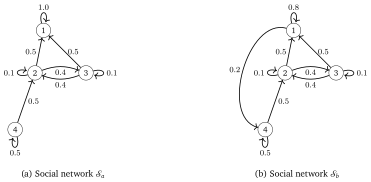
Figure 4.13:Two social networks
Figure 4.13 shows two social networks and with trust matrices given by
respectively. In network A, agent 1 places no trust in anyone’s opinion but his own. In network B, he places at least some trust in the opinion of agent 4. Below we show how these differences matter for the dynamics of beliefs.
4.2.4.1Learning
At time zero, all agents have an initial subjective belief concerning the validity of a given statement. Belief takes values in , with 1 indicating complete (subjective) certainty that the statement is true. Let be the belief of agent at time zero.
An agent updates beliefs sequentially based on the beliefs of others, weighted by the amount of trust placed in their opinion. Specifically, agent updates her belief after one unit of time to . More generally, at time , beliefs update to
In matrix notation this is , where each is treated as a column vector.
(Notice that this update rule is similar but not identical to the marginal distribution updating rule for Markov chains (the forward equation) discussed. Here we are postmultiplying by a column vector rather than premultiplying be a row vector.)
4.2.4.2Consensus
A social network is said to lead to consensus if as for all . Consensus implies that all agents eventually share the same belief. An important question is, what conditions on the network lead to a consensus outcome?
Proposition 4.2.6 can be applied to the two social networks and in Figure 4.13. For example, in network , for every node , there exists a walk of length 2 from to node . Hence, by Lemma 4.2.5, we have . In network the same is true.
4.2.4.3Influence of Authorities
Now let’s consider what beliefs converge to when consensus emerges. In particular, we are interested in discovering whose opinions are most influential under De Groot learning, for a given trust matrix.
To answer the question, let be a given social network with trust matrix . Suppose that for some . By Theorem 4.2.4, the network is globally stable when viewed as a finite Markov model. Let be the unique stationary distribution, so that .
Applying (4.34) with and yields
where
We conclude that the belief of every agent converges geometrically to , which is a weighted average of the initial beliefs of all agents. In particular, those agents with high weighting under the stationary distribution have a large influence on these equilibrium beliefs.
We can interpret this through notions of centrality. Since , we have , so is the authority-based eigenvector centrality measure on . Thus, the influence of each agent on long run beliefs is proportional to their authority-based eigenvector centrality. This makes sense because such agents are highly trusted by many agents who are themselves highly trusted.
4.3Chapter Notes
High quality treatments of finite-state Markov dynamics include Norris (1998), Privault (2013) and Häggström (2002). For the general state case see Meyn & Tweedie (2009).
A review of De Groot learning is available in Jackson (2010). Some interesting extensions related to the “wisdom of crowds” phenomenon are provided in Golub & Jackson (2010). Molavi et al. (2018) provide a theory of social learning that includes De Groot learning as a special case. Acemoglu et al. (2021) study misinformation and echo chambers in information networks. Board & Vehn (2021) analyze learning dynamics in continuous time on large social networks. Shiller (2020) provides an interesting discussion of how ideas spread across social networks and shape economic outcomes. In a large-scale empirical study, Chetty et al. (2022) analyze how cross-class friendships influence social mobility. Acemoglu et al. (2023) consider the effect of strong and weak links on Bayesian learning in a social network. Dasaratha et al. (2022) analyze how Bayesian agents learn about a changing state by interacting with their neighbors. While the resulting dynamics are similar to those of the De Groot model, they are generated as an equilibrium outcome rather than imposed as a behavioral assumption.
Example 4.1.2 is intended as an illustration of the mechanics of updating distributions. While the methodology in Quah (1993) is thought provoking, it struggles to make plausible long run predictions about something as complex as the cross-country income distribution. Indeed, the Kullback–Leibler deviation between the predicted and realized 2019 distributions is actually larger than the Kullback–Leibler deviation between the 1985 and 2019 distributions. Evidently, a naive estimate “nothing will change” model predicts better than Quah’s. Most of the focus in this text is on short term forecasts and scenarios, where the system is approximately stationary after suitable transformations, rather than heroic long term predictions where nonstationary change is hard to quantify.
There are many useful extensions to Brouwer’s theorem, such as one for set-valued functions due to Kakutani (1941). These results have many applications in economics (see, for example, Nash (1950)). Another paper, due to Schauder (1930), extends Brouwer’s result to infinite dimensional spaces.
Seneta (2006) also discusses the history of Andrey Markov’s work, which originated the kinds of contraction based arguments used in this section.
It can be shown that the condition for some is necessary as well as sufficient for global stability of a finite Markov model. Hence the conditions of Theorem 4.2.4 are strictly weaker than strong connectedness plus aperiodicity, as used in Theorem 4.1.1.
- Quah, D. (1993). Empirical cross-section dynamics in economic growth. European Economic Review, 37(2-3.), 426–434.
- Benhabib, J., Bisin, A., & Luo, M. (2019). Wealth distribution and social mobility in the US: A quantitative approach. American Economic Review, 109(5), 1623–1647.
- Aliprantis, C. D., & Border, C., Kim. (1999). Infinite dimensional analysis: a hitchhiker’s guide (2nd ed.). Springer-Verlag, New York.
- Meyn, S. P., & Tweedie, R. L. (2009). Markov chains and stochastic stability. Cambridge University Press.
- Stachurski, J. (2022). Economic dynamics: theory and computation (2nd ed.). MIT Press.
- Seneta, E. (2006). Markov and the creation of Markov chains. Markov Anniversary Meeting, 1–20.
- DeGroot, M. H. (1974). Reaching a consensus. Journal of the American Statistical Association, 69(345), 118–121.
- Norris, J. R. (1998). Markov chains. Cambridge university press.
- Privault, N. (2013). Understanding Markov Chains. Examples and Applications, Publisher Springer-Verlag Singapore, 357, 358.
- Häggström, O. (2002). Finite Markov chains and algorithmic applications. Cambridge University Press.
- Jackson, M. O. (2010). Social and economic networks. Princeton university press.
- Golub, B., & Jackson, M. O. (2010). Naive learning in social networks and the wisdom of crowds. American Economic Journal: Microeconomics, 2(1), 112–149.
- Molavi, P., Tahbaz-Salehi, A., & Jadbabaie, A. (2018). A theory of non-Bayesian social learning. Econometrica, 86(2), 445–490.
- Acemoglu, D., Ozdaglar, A., & Siderius, J. (2021). Misinformation: Strategic Sharing, Homophily, and Endogenous Echo Chambers [Techreport]. National Bureau of Economic Research.
- Board, S., & Meyer-ter Vehn, M. (2021). Learning dynamics in social networks. Econometrica, 89(6), 2601–2635.