Up until now we have analyzed problems where network structure is either fixed or generated by some specified random process. In this chapter, we investigate networks where connections are determined endogenously via equilibrium or optimality conditions. In the process, we cover some of the most powerful methods available for solving optimization problems in networks and beyond, with applications ranging from traditional graph and network problems, such as trade, matching, and communication, through to machine learning, econometrics and finance.
3.1Shortest Paths
As a preliminary step, we study the shortest path problem—a topic that has applications in production, network design, artificial intelligence, transportation and many other fields. The solution method we adopt also happens to be one of the clearest illustrations of Bellman’s principle of optimality, which is one of the cornerstones of optimization theory and modern economic analysis.
3.1.1Definition and Examples
We start proceedings by introducing simple examples. (In the next section we will formalize the problem and consider solution methods.)
3.1.1.1Set Up
Consider a firm that wishes to ship a container from to at minimum cost, where and are vertices of the weighted digraph shown in Figure 3.1. Arrows (edges) indicate paths that can be used for freight, while weights indicate costs of traversing them. In this context, the weight function is also called the cost function, and we denote it by . For example, is the cost of traveling from vertex to vertex .
Since this graph is small, we can find the minimum cost path visually. A quick scan shows that the minimum attainable cost is 8. Two paths realize this cost: and , as shown in Figure 3.2 and Figure 3.3, respectively.
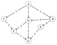
Figure 3.1:Graph for the shortest path problem
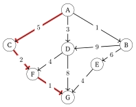
Figure 3.2:Solution 1
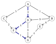
Figure 3.3:Solution 2
3.1.1.2A Recursive View
Let’s now consider a systematic solution that can be applied to larger graphs. Let denote the minimum cost-to-go from vertex . That is, is the total cost of traveling from to if we take the best route. Its values are shown at each vertex in Figure 3.4. We can represent in vector form via
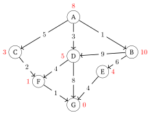
Figure 3.4:The cost-to-go function, with indicated by red digits at each
As is clear from studying Figure 3.4, once is known, the least cost path can be computed as follows: Start at and, from then on, at arbitrary vertex , move to any that solves
Here is the set of direct successors of , as defined in Section 1.4.1, while is the cost of traveling from to . In other words, to minimize the cost-to-go, we choose the next path to minimize current traveling cost plus cost-to-go from the resulting location.
Thus, if we know at each , then finding the best path reduces to the simple two stage optimization problem in (3.2).
But now another problem arises: how to find in more complicated cases, where the graph is large? One approach to this problem is to exploit the fact that
must hold for every vertex in the graph apart from (where ).
Take the time to convince yourself that, for our example, the function satisfies (3.3). In particular, check that (3.3) holds at each nonterminal in Figure 3.4.
We can understand (3.3), which is usually called the Bellman equation, as a restriction on that helps us identify this vector. The main difficulty with our plan is that the Bellman equation is nonlinear in the unknown function . Our strategy will be to convert this nonlinear equation into a fixed point problem, so that fixed point theory can be applied.
We do this in the context of a more general version of the shortest path problem.
3.1.2Bellman’s Method
We consider a generic shortest path problem on a flow network, which consists of a weighted digraph with a sink called the destination and a weight function that associates a positive cost to each edge . In what follows we take .
We consider how to find the shortest (i.e., minimum cost) path from to for every . In doing so we impose the following assumption.
To simplify the arguments below, we consider a second digraph where is unchanged and . In other words, extends by adding a self-loop at . We also extend to this self-loop by setting . This just means that “terminating at ” is the same as “staying at ,” since no more cost accrues after arrival at the destination. Figure 3.5 illustrates in the context of the previous example.
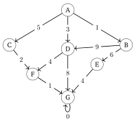
Figure 3.5:Addition of a self loop to the destination
We will use the intuition from the previous section, based around the Bellman equation, to construct a solution method.
3.1.2.1Policies
Instead of optimal paths, it turns out to be more convenient to aim for optimal policies. In general, a policy is a specification of how to act in every state. In the present setting, a policy is a map with understood as meaning “when at vertex , go to .” A policy is called feasible if for all .
For any feasible policy and , the trajectory of under is the path from to the destination indicated by the feasible policy. In other words, it is the sequence defined by and for all . It can also be expressed as , where is the -th composition of with itself.
Let be the set of all feasible policies. In view of Exercise 3.1.1, policies in have the property that every trajectory they generate reaches in steps and stays there. In other words,
Given , we call -greedy if
In essence, a greedy policy treats as the minimum cost-to-go function and picks out an optimal path under that assumption.
Using our new terminology, we can rephrase the discussion in Section 3.1.1.2 as follows: the shortest path problem can be solved by finding the true minimum cost-to-go function and then following a -greedy policy. In the remainder of this section, we prove this claim more carefully.
3.1.2.2Cost of Policies
We need to be able to assess the cost of any given policy. To this end, for each and , let denote the cost of following from . That is,
This second equality holds because for all and . The function is called the cost-to-go under .
It will be helpful in what follows to design an operator such that is a fixed point. For this purpose we let be all with and define by
Here and below, with , the expression indicates the -th composition of with itself (i.e., is applied times).
3.1.2.3Optimality
The minimum cost-to-go function is defined by
The definition of matches our intuitive definition from Section 3.1.1.2, in the sense that is, for each , the minimum cost of traveling from to the destination .
A policy is called optimal if it attains the minimum in the definition of , so that on . Our main aims are to
obtain a method for calculating and
prove that a -greedy policy is optimal, as suggested in our informal discussion above.
Regarding the first step, we claim that satisfies the Bellman equation (3.3). To prove this claim we introduce the Bellman operator via
By construction, satisfies the Bellman equation (3.3) if and only if .
The next result is central. It confirms that the minimum cost-to-go function satisfies the Bellman equation and also provides us with a means to compute it: pick any in and then iterate with .
We now have a means to compute the minimum cost-to-go function (by iterating with , starting at any ) and, in addition, a way to verify the following key result.
3.1.2.4An Implementation in Julia
Let’s use the ideas set out above to solve the original shortest path problem, concerning shipping, which we introduced in Section 3.1.1.1. We will implement in Julia.
Our first step is to set up the cost function, which we store as an array called c. We identify the vertices , ..., , with the integers . We set c[i, j] = Inf when no edge exists from i to j, so that such a path is never chosen when evaluating the Bellman operator, as defined in (3.3). When an edge does exist, we enter the cost shown in Figure 3.1.
c = fill(Inf, (7, 7))

c[1, 2], c[1, 3], c[1, 4] = 1, 5, 3
c[2, 4], c[2, 5] = 9, 6
c[3, 6] = 2
c[4, 6] = 4
c[5, 7] = 4
c[6, 7] = 1
c[7, 7] = 0
Next we define the Bellman operator:
function T(q)
    Tq = similar(q)
    n = length(q)
    for x in 1:n
        Tq[x] = minimum(c[x, :] + q[:])
    end
    return Tq
end
Now we arbitrarily set , generate the sequence of iterations and plot them:
using PyPlot
fig, ax = plt.subplots()

n = 7
q = zeros(n)
ax.plot(1:n, q)

for i in 1:3
    new_q = T(q)
    ax.plot(1:n, new_q, "-o", alpha=0.7)
    global q = new_q
end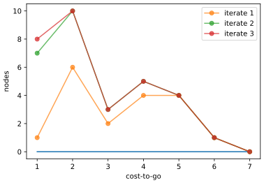
Figure 3.6:Shortest path Bellman iteration
After adding some labels, the output looks like the image in Figure 3.6. Notice that, by , we have already converged on . You can confirm this by checking that the values of line up with those we obtained manually in Figure 3.4.
3.1.3Betweenness Centrality
In Section 1.4.3 we discussed a range of centrality measures for networks, including degree, eigenvector and Katz centrality. Aside from these, there is another well-known centrality measure, called betweenness centrality, that builds on the notion of shortest paths and is particularly popular in analysis of social and peer networks.
Formally, for a given graph , directed or undirected, the betweenness centrality of vertex is
where is the set of all shortest paths from to and is the set of all shortest paths from to that pass through . (As usual, is the cardinality of .) Thus, is proportional to the probability that, for a randomly selected pair of nodes , a randomly selected shortest path from to contains . Thus, the measure will be high for nodes that “lie between” a large number of node pairs.
For example, Networkx stores a graph called florentine_families_graph that details the marriage relationships between 15 prominent Florentine families during the 15th Century. The data can be accessed via
import networkx as nx
G = nx.florentine_families_graph()
The network is shown in Figure 3.7, which was created using
nx.draw_networkx(G, [params]) where [params] stands for parameters listing node size, node color and other features. For this graph, node size and node color are scaled by betweenness centrality, which is calculated via
nx.betweenness_centrality(G) Although this graph is very simple, the output helps to illustrate the prominent role of the Medici family, consistent with their great wealth and influence in Florence and beyond.
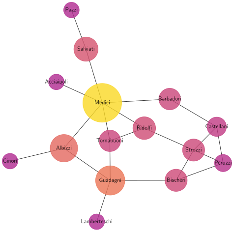
Figure 3.7:Betweenness centrality (by color and node size) for Florentine families
3.2Linear Programming and Duality
Our study of shortest paths in Section 3.1 used a relatively specialized optimization method. In this section we cover more general results in optimization and duality, which will then be applied to endogenous networks, optimal transport and optimal flows. Part of the strategy is to take challenging optimization problems and regularize them, often by some form of convexification.
Before diving into theory, we use Section 3.2.1 below to provide motivation via one very specific application. This application involves what is typically called matching in economics and linear assignment in mathematics. We illustrate the key ideas in the context of matching workers to jobs. Later, when we discuss how to solve the problem, we will see the power of linear programming, convexification and duality.
3.2.1Linear Assignment
Behold the town of Springfield. A local employer is shutting down and 40 workers stand idled. Fortunately for these workers, Springfield lies within a political battleground state and, as a result, the mayor receives backing to attract a new employer. She succeeds by promising a certain firm that the 40 workers will be retrained for the new skills they require. For mathematical convenience, let us suppose that there are exactly 40 new positions, each with distinct skill requirements.
The team set up by the mayor records the individual skills of the 40 workers, along with the requirements of the new positions, and estimates the cost of retraining individual for position . The team’s challenge is to minimize the total cost of retraining. In particular, they wish to solve
where is the set of all permutations (i.e., bijective self-maps) on the integers . Figure 3.8 illustrates one possible permutation.
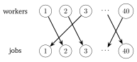
Figure 3.8:One possible assignment (i.e., permutation of )
The problem is discrete, so first order conditions are unavailable. Unsure of how to proceed but possessing a powerful computer, the team instructs its workstation to step through all possible permutations and record the one that leads to the lowest total retraining cost. The instruction set is given in Algorithm 2.
After five days of constant execution, the workstation is still running and the mayor grows impatient. The team starts to calculate how long execution will take. The main determinant is the size of the set . Elementary combinatorics tells us that the number of permutations of a set of size is . Quick calculations show that exceeds . A helpful team member points out that this is much less than the number of possible AES-256 password keys (approximately ). The mayor is not appeased and demands a runtime estimate.
Further calculations reveal the following: if, for each in , the workstation can evaluate the cost in -th of a second (which is extremely optimistic), then the total run time would be
Another helpful team member provides perspective by noting that the sun will expand into a red giant and vaporize planet Earth in less than years.
The great computational cost of solving this problem by direct calculations is an example of what is often called the curse of dimensionality. This phrase, coined by Richard Bellman (1920-1984) during his fundamental research into dynamic optimization, refers to the exponential increase in processor cycles needed to solve computational problems to a given level of accuracy as the number of dimensions increases. The matching problem we have just described is high-dimensional because the choice variable , a permutation in , is naturally associated with the vector . This, in turn, is a point in 40-dimensional vector space.[1]
Fortunately, clever algorithms for this matching problem have been found and, for problems such as this one, useful approximations to the optimal allocation can be calculated relatively quickly. For example, Dantzig (1951) showed how such problems can be cast as a linear program, which we discuss below. Further progress has been made in recent years by adding regularization terms to the optimization problem that admit derivative-based methods.
In the sections that follow, we place matching problems in a more general setting and show how they can be solved efficiently. Our first step is to review the basics of linear programming.
3.2.2Linear Programming
A linear program is an optimization problem with a linear objective function and linear constraints. If your prior belief is that all interesting problems are nonlinear, then let us reassure you that linear programming is applicable to a vast array of interesting applications. One of these is, somewhat surprisingly, the assignment problem in Section 3.2.1, as famously demonstrated by the American mathematician George Bernard Dantzig (1914–2005) in Dantzig (1951). Other applications include optimal flows on networks and optimal transport problems, which in turn have diverse applications in economics, finance, engineering and machine learning.
We explain the key ideas below, beginning with an introduction to linear programming.
3.2.2.1A Firm Problem
One way to define linear programs is in terms of what open source and commercial solvers for linear programming problems handle. Typically, for these solvers, the problem takes the form
Here each is a matrix with columns and and are conformable column vectors.
To illustrate, let’s consider a simple example, which concerns a firm that fabricates products labeled . To make each product requires machine hours and labor. Product requires machine hours and labor hours per unit of output, as shown in the table below
| product | machine hours | labor hours | unit price |
|---|---|---|---|
| 1 | |||
A total of machine hours and labor hours are available. Letting denote output of product , the firm’s problem is
subject to
Here is profits and and are the wage rate and rental rate of capital. We are taking these values as fixed, along with and , so choosing the that maximizes profits is the same as choosing the that maximizes revenue . This will be our objective in what follows.
(Why are total labor supply and machine hours held fixed here? We might think of this problem as one of designing a daily or weekly production plan, which optimally allocates existing resources, given current prices.)
Figure 3.9 shows an illustration of a simple case with two products. Consistent with Exercise 3.2.3, the feasible set is a polyhedron, shaded in blue. The green lines are contour lines of the revenue function , with and . By inspecting this problem visually, and recognizing that the contour lines are increasing as we move to the northeast, it is clear that the maximum is obtained at the extreme point indicated in the figure.
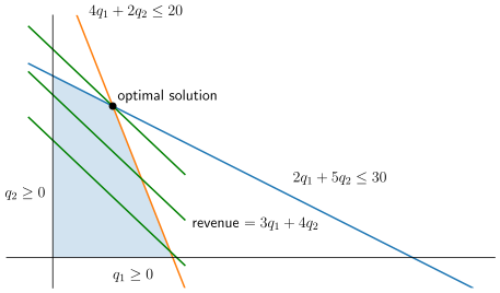
Figure 3.9:Revenue maximizing quantities
Maximizing revenue is equivalent to minimizing , so with we have a linear programming problem to which we can apply a solver.
3.2.2.2A Python Implementation
Let’s look at one option for solving this problem with Python, via SciPy’s open source solver linprog. For the simple two-product firm problem, we ignore the unnecessary equality constraint in (3.9) and set
The bound is imposed by default so we do not need to specify and .
We apply the numbers in Figure 3.9, so the maximization version of the problem is
Now we set up primitives and call linprog as follows:
A = ((2, 5),
     (4, 2))
b = (30, 20)
c = (-3, -4)  # minus in order to minimize

from scipy.optimize import linprog
result = linprog(c, A_ub=A, b_ub=b)
print(result.x)
The output is [2.5, 5.0], indicating that we should set and . The result is obtained via the simplex algorithm, discussed in Section 3.2.2.8.
3.2.2.3A Julia Implementation
When solving linear programs, one option is to use a domain specific modeling language to set out the objective and constraints in the optimization problem. In Python this can be accomplished using the open source libraries such as Pyomo and Google’s OR-Tools. In Julia we can use JuMP.
The following code illustrates the Julia case, using JuMP, applied to the firm problem (3.11).
using JuMP
using GLPK

m = Model()
set_optimizer(m, GLPK.Optimizer)

@variable(m, q1 >= 0)
@variable(m, q2 >= 0)
@constraint(m, 2q1 + 5q2 <= 30)
@constraint(m, 4q1 + 2q2 <= 20)
@objective(m, Max, 3q1 + 4q2)

optimize!(m)
Notice how the JuMP modeling language allows us to write objectives and constraints as expressions, such as 2q1 + 5q2 <= 30. This brings the code closer to the mathematics and makes it highly readable.
If we now run value.(q1) and value.(q2), we get 2.5 and 5.0, respectively, which are the same as our previous solution.
3.2.2.4Standard Linear Programs
The programming problem in (3.8)–(3.9) is convenient for applications but somewhat cumbersome for theory. A more canonical version of the linear programming problem is
Here is interpreted as a column vector in , is also a column vector in , is , and is . A linear program in the form of (3.12) is said to be in standard equality form. In preparation for our discussion of duality below, we also call (3.12) the primal problem.
Standard equality form is more general than it first appears. In fact the original formulation (3.8)–(3.9) can be manipulated into standard equality form via a sequence of transformations. Hence, when treating theory below, we can specialize to standard equality form without losing generality.
Although we omit full details on the set of necessary transformations (which can be found in Bertsimas & Tsitsiklis (1997) and many other sources), let’s gain some understanding by converting the firm optimization problem into standard equality form. To simplify notation, we address this task when , although the general case is almost identical.
As above, we switch to minimization of a linear constraint by using the fact that maximizing revenue is equivalent to minimizing . Next, we need to convert the two inequality constraints (3.10) into equality constraints. We do this by introducing slack variables and and rewriting the constraints as
Indeed, we can see that requiring and is the same as imposing , and the same logic extends to the labor constraint.
Setting , we can now express the problem as
subject to
This is a linear program in standard equality form.
3.2.2.5Duality for Linear Programs
One of the most important facts concerning linear programming is that strong duality always holds. Let us state the key results. The dual problem corresponding to the standard equality form linear program (3.12) is
Readers who have covered Section 6.1.7 in the appendix will be able to see the origins of this expression. In particular, by formula (6.19) in the appendix, the dual problem corresponding to the standard equality form linear program (3.12) can be expressed as
and . (We can also treat the inequality via a multiplier but this turns out to be unnecessary.) Now observe that
Since the dual problem is to maximize this expression over , we see immediately that a violating will never be chosen. Hence the dual to the primal problem (3.12) is (3.13).
3.2.2.6Strong Duality
As shown in Section 6.1.7.1 of the appendix, the inequality always holds, where is the primal value in (3.12). This is called weak duality. If , then strong duality is said to hold. Unlike weak duality, strong duality requires conditions on the primitives.
The next theorem states that, for linear programs, strong duality holds whenever a solution exists. A proof can be obtained either through Dantzig’s simplex method or via Farkas’ Lemma. See, for example, Ch. 4 of Bertsimas & Tsitsiklis (1997) or Ch. 6 of Matousek & Gärtner (2007).
Strong duality of linear programs has many important roles. Some of these are algorithmic: duality can be used to devise efficient solution methods for linear programming problems. Another way that duality matters for economists is that it provides deep links between optimality and competitive equilibria, as we show below.
3.2.2.7Complementary Slackness
We say that and satisfy the complementary slackness conditions for the linear program (3.12) when
While it is possible to derive these expressions from the complementary slackness in the KKT conditions in Section 6.1.7.3, a better approach is to connect them directly to the saddle point condition.
To see how this works, suppose that is feasible for the primal problem and is feasible for the dual problem. If is a saddle point of , then the complementary slackness conditions (3.15)–(3.16) must hold. Indeed, (3.15) is trivial when is feasible, since . At the same time, (3.16) must be true because violation implies that
due to dual feasibility (i.e., ) and . But then is not a saddle point of , since changing the -th element of to zero strictly reduces the Lagrangian
By sharpening this argument, it is possible to show that, for linear programs, the complementary slackness conditions are exact necessary and sufficient conditions for a saddle point of the Lagrangian. This leads to the next theorem.
Chapter 4 of Bertsimas & Tsitsiklis (1997) provides more discussion and a full proof of Theorem 3.2.2. Below, we illustrate some of the elegant connections between complementary slackness and equilibria in competitive economic environments.
3.2.2.8The Simplex Algorithm
Linear programming is challenging in high-dimensional settings, partly because the linear objective function implies that solutions are not interior. The first efficient solution methods for linear programs appeared in the 1930s and 1940s, starting with the simplex method of Kantorovich and Dantzig. As the simplex method began to prove its worth, linear programming grew into a technique of enormous practical importance. Operations research, communication and production systems began to make heavy use of linear programs.
The simplex algorithm makes use of the following result, which is proved in Theorem 2.7 of Bertsimas & Tsitsiklis (1997).
(An extreme point of a polyhedron was defined in Section 6.1.5.1. The feasible set was shown to be a polyhedron in Exercise 3.2.3.)
The simplex algorithm makes use of Theorem 3.2.3 by walking along edges of the polyhedron that forms the feasible set, from one extreme point to another, seeking at each step a new extreme point (which coincides with a vertex of the polyhedron) that strictly lowers the value of the objective function. Details can be found in Bertsimas & Tsitsiklis (1997) and Matousek & Gärtner (2007).
3.3Optimal Transport
Next we turn to optimal flows across networks. One simple—but computationally nontrivial—example of a network flow problem is the linear assignment problem we analyzed in Section 3.2.1. There, the vertices are either workers or jobs and the edges are assignments, chosen optimally to minimize aggregate cost. More general network flow problems extend these ideas, allowing endogenous formation of networks in more sophisticated settings. The general structure is that vertices are given, while edges and weights are chosen to optimize some criterion. There are natural applications of these ideas in trade, transportation and communication, as well as less obvious applications within economics, finance, statistics and machine learning.
In our study of network flows, we begin with the optimal transport problem, which is the most important special case of the general network flow problem. (In fact, as we show in Section 3.3.4.3, there exists a technique by which the general network flow problem can always be reduced to an optimal transport problem.)
3.3.1The Monge-Kantorovich Problem
Optimal transport is a classic problem dating back to the work of Gaspard Monge (1746–1818), who studied, among many other things, the transport of earth for construction of forts. This simple-sounding problem—how to transport a pile of given shape into a new pile of given shape at minimum cost—can, after normalization, be identified with the problem of least cost transformation of one distribution into another distribution. Figure 3.10 gives a visualization of transforming one distribution into another in one dimension (although the cost function is not specified).
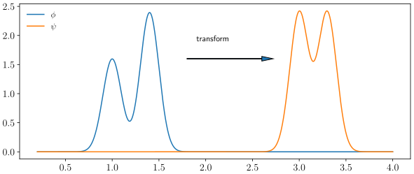
Figure 3.10:Transforming distribution into distribution
It turns out that, by varying the notion of cost, this transportation problem provides a highly flexible method for comparing the distance between two distributions, with the essential idea being that distributions are regarded as “close” if one can be transformed into the other at low cost. The resulting distance metric finds wide-ranging and important applications in statistics, machine learning and various branches of applied mathematics.[2]
In economics, optimal transport has important applications in transportation and trade networks, as well as in matching problems, econometrics, finance and so on (see, e.g., Galichon (2018)). As such, it is not surprising that economists have contributed a great deal to the optimal transport problem, with deep and fundamental work being accomplished by the great Russian mathematical economist Leonid Kantorovich (1912–1986), as well as the Dutch economist Tjalling Koopmans (1910–1985), who shared the Nobel Prize with Kantorovich in 1975 for their work on linear programming and optimal transport.[3]
We start our discussion with a straightforward presentation of the mathematics. Then, in Section 3.3.3, we will connect the mathematics to economic problems, and show the deep connections between transport, duality, complementary slackness and competitive equilibria.
3.3.1.1Monge’s Formulation
We start with the classical problem of Monge, which is simple to explain. We take as given two finite sets and , paired with distributions and . Elements of and are called locations. To avoid tedious side cases, we assume throughout that and are strictly positive on their domains. In addition, we are supplied with a cost function . Our goal is to “transport” into at minimum cost. That is, we seek to solve
over the set of all maps from onto satisfying
The constraint says must be such that, for each target location , the sum of all probability mass sent to is equal to the specified quantity . The symbol is short for . In this context, is often called a Monge map.
The problem is easily illustrated in the current discrete setting. Figure 3.11 gives a visualization when locations are enumerated as and , with both and being subsets of . For simplicity, is written as and similarly for . Vertex size is proportional to probability mass assigned to the vertex. The edges represent one feasible Monge map.
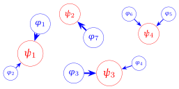
Figure 3.11:A Monge map transporting ϕ to ψ
Discreteness and lack of convexity in the constraint (3.18) imply that the Monge problem is, in general, hard to solve. Truly fundamental progress had to wait until Kantorovich showed how convexification can greatly simplify the problem. The convexification process requires shifting the problem to a higher dimensional space, but the cost of higher dimensions is outweighed by the regularization provided by convexity and lack of discreteness. We study the Kantorovich formulation in Section 3.3.1.3.
3.3.1.2Assignment as Optimal Transport
The linear assignment problem studied in Section 3.2.1, with cost of training worker for job , is a special case of optimal transport. All we have to do is set and take and to be discrete uniform distributions on .
Since must be a bijection on , which is also a permutation of , the objective of the optimal transport problem under the current configuration is
where is the set of all permutations of . This is the same optimization problem as the linear assignment problem in (3.7).
3.3.1.3Kantorovich’s Relaxation of the Monge Problem
The basic idea in Kantorovich’s relaxation of the Monge problem is to allow mass located at arbitrary to be mapped to multiple locations in , rather than just one. This means that we are no longer seeking a function , since, by definition, a function can map a given point to only one image. Instead, we seek a “transport plan” that sends some fraction of the mass at to . The plan is constrained by the requirement that, for all and ,
total probability mass sent to is and
total probability mass sent from is .
These constraints on this transport plan mean that it takes the form of a “coupling,” which we define below.
Figure 3.12 illustrates a feasible transport plan in the discrete setting. As with Figure 3.11, is written as and similarly for , while vertex size is proportional to probability mass. Unlike the Monge setting of Figure 3.11, the mass at each vertex can be shared across multiple , as long as the constraints are respected.
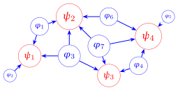
Figure 3.12:Kantorovich relaxation of the Monge problem
Let’s write the constraints more carefully. We recall that, in probability theory, a coupling is a joint distribution with specific marginals. More precisely, given in and in , a coupling of is an element of with marginals and . This restriction on marginals means that
The constraints in (3.20)–(3.21) require that
for any , the total amount of probability mass flowing out of is and
for any , the total amount of probability mass flowing into is .
In the present setting, a coupling is also called a transport plan.
Let be the set of all couplings of and . Taking and the cost function as given, the general Monge–Kantorovich problem, also called the optimal transport problem, is to solve
where
is the Frobenius inner product of and , treated as matrices. The sum in measures the total cost of transporting into under the plan . There is linearity embedded in this cost formulation, since doubling the amount sent from to scales the associated cost at rate .
We call any solving (3.22) an optimal plan. Since we are maximizing over a finite set, at least one such plan exists.
3.3.1.4Optimal Transport as a Linear Program
With some relatively simple manipulations, the general optimal transport problem can be mapped into a standard equality form linear program. This provides two significant benefits. First, we can apply duality theory, which yields important insights. Second, on the computational side, we can use linear program solvers to calculate optimal plans.
To map the optimal transport problem into a linear program, we need to convert matrices into vectors. Will use the operator, which takes an arbitrary and maps it to a vector in by stacking its columns vertically. For example,
In this section we adopt the notational conventions in Exercise 3.3.5. The objective function for the optimal transport problem can now be expressed as .
To rewrite the constraints in terms of , we use the Kronecker product, which is denoted by and defined as follows. Suppose is an matrix with entries and that is an matrix. The Kronecker product of and is the matrix defined, in block matrix form, by
It can be shown that Kronecker products and the operator are connected by the following relationship: for conformable matrices , and , we have
Using (3.24) and the symbol for the identity matrix, we can rewrite the first constraint in (3.23) as
Now, using block matrix notation and setting
the optimal transport problem can be expressed as the standard equality form linear program
Finally, for a given solution , the transport plan is recovered by inverting .
3.3.1.5Implementation
Listing 1 is a function that implements the above steps, given flat (one-dimensional) arrays phi and psi representing the distributions over the source and target locations, plus a two-dimensional array c representing transport costs. (The method argument highs-ipm tells linprog to use a particular interior point method, details of which can be found in the linprog documentation. Simplex and other methods give similar results.)
import numpy as np
from scipy.optimize import linprog

def ot_solver(phi, psi, c, method='highs-ipm'):
    """
    Solve the OT problem associated with distributions phi, psi
    and cost matrix c.

    Parameters
    ----------
    phi : 1-D array
        Distribution over the source locations.
    psi : 1-D array
        Distribution over the target locations.
    c : 2-D array
        Cost matrix.
    """
    n, m = len(phi), len(psi)

    # vectorize c
    c_vec = c.reshape((m * n, 1), order='F')

    # Construct A and b
    A1 = np.kron(np.ones((1, m)), np.identity(n))
    A2 = np.kron(np.identity(m), np.ones((1, n)))
    A  = np.vstack((A1, A2))
    b  = np.hstack((phi, psi))

    # Call solver
    res = linprog(c_vec, A_eq=A, b_eq=b, method=method)

    # Invert the vec operation to get the solution as a matrix
    pi = res.x.reshape((n, m), order='F')
    return pi
Listing 1:Function to solve a transport problem via linear programming
Notice that in Listing 1, the reshape order is specified to F. This tells NumPy to reshape with Fortran column-major order, which coincides with the definition of the operator described in Section 3.3.1.4. (The Python vectorize operation defaults to row-major order, which concatenates rows rather than stacking columns. In contrast, Julia uses column-major by default.)
Let’s call this function for the very simple problem
With these primitives, all mass from and should be sent to . To implement this problem we set
phi = np.array((0.5, 0.5))
psi = np.array((1, 0))
c = np.ones((2, 2))
and then call ot_solver via
ot_solver(phi, psi, c)The output is as expected:
array([[0.5, 0. ],
[0.5, 0. ]]) 3.3.1.6Python Optimal Transport
In the case of Python, the steps above have been automated by the Python Optimal Transport package, due to Flamary et al. (2021). For the simple problem from Section 3.3.1.5 we run
import ot
ot.emd(phi, psi, c)   # Use simplex method via the emd solver
The output is again equal to
array([[0.5, 0. ],
       [0.5, 0. ]])
Figure 3.13 shows an example of an optimal transport problem solved using the Python Optimal Transport package. The interpretation is similar to Figure 3.12, although the number of vertices is larger. In addition, the edges show the optimal transport configuration, in the sense that , the optimal transport plan, is treated as the adjacency matrix for the graph. (The figure shows the unweighted graph, with an arrow drawn from to whenever .) The optimal transport plan is obtained by converting the transport problem into a linear program, as just described, and applying the simplex method. Although there are 32 nodes of each type, the problem is solved by the simplex routine in less than one millisecond.
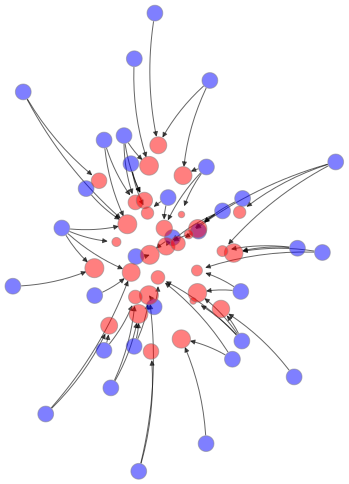
Figure 3.13:An optimal transport problem solved by linear programming
3.3.1.7Kantorovich Relaxation and Linear Assignment
We showed in Section 3.3.1.2 that the linear assignment problem studied in Section 3.2.1 is a special case of optimal transport, where and become discrete uniform distributions on . Moreover, as we have just seen, Kantorovich’s relaxation method allows us to apply linear programming. This leads to fast solutions.
In the discussion in Section 3.2.1 we used . Let’s start here with , to illustrate the method, and then try with . The matrix of costs, which is the only other primitive, will be generated randomly as an independent array of uniform random variables: Then we apply the Python Optimal Transport (POT) library, as in Section 3.3.1.6.
Here is our set up:
import numpy as np
import ot

n = 4
phi = np.ones(n)
psi = np.ones(n)
We have broken the rule that and should sum to one. This could be fixed easily by using np.ones(n)/n instead of np.ones(n), but the POT library does not care (as long as np.sum(phi) equals np.sum(psi)) and, moreover, the idea of putting unit mass everywhere is natural, since each element of represents one worker, and each element of represents one job.
Now we build the cost matrix:
c = np.random.uniform(size=(n, n))The output is
array([[0.03841, 0.32896, 0.55989, 0.41682],
       [0.91527, 0.24566, 0.26022, 0.64510],
       [0.96275, 0.44089, 0.79274, 0.93065],
       [0.40454, 0.87307, 0.43555, 0.54903]])
(For example, the cost of retraining worker 1 for job 2 is 0.32896.) Finally, we call the solver:
ot.emd(phi, psi, c) The output is
array([[1., 0., 0., 0.],
       [0., 0., 1., 0.],
       [0., 1., 0., 0.],
       [0., 0., 0., 1.]])
This is a permutation matrix, which provides another way to express a permutation of . The first row tells us that worker 1 is assigned to job 1, the second tells us that worker 2 is assigned to job 3, and so on.
If we now set and rerun the code, the line ot.emd(phi, psi, c), which calls the simplex-based solver, runs in less than 1 millisecond on a mid-range laptop. This is a remarkable improvement on the year estimate for the brute force solver we obtained in Section 3.2.1.
3.3.1.8Tight Relaxation
Notice that the solution we obtained for the linear assignment problem using the simplex method does not split mass, as permitted by the Kantorovich relaxation. For example, we do not send half of a worker to one job and the other half to another. This is convenient but why does it hold?
While we omit the details, the basic idea is that a general Kantorovich transport plan is a bistochastic matrix, and all such matrices can be formed as convex combinations of permutation matrices. (This is called Birkhoff’s Theorem.) In other words, the permutation matrices are extreme points of the set of bistochastic matrices. Moreover, Theorem 3.2.3 tells us that any optimizer of a linear program will be an extreme point—in this case, a permutation matrix.
3.3.2Kantorovich Duality
One of the greatest achievements of Kantorovich was to show that the optimal transport problem can be connected to a dual problem, and how that dual problem can be used to characterize solutions. This work anticipated much of the later development of duality theory for arbitrary linear programs.
Throughout this section, in stating the main results, we use the notation
This is just the usual inner product, when we think of and as vectors in . Also, given a cost function on , let be all pairs in such that
One part of Kantorovich’s duality results runs as follows.
Theorem 3.3.1 can now be understood as a special case of the more general result that strong duality holds for linear programs, which we stated in Theorem 3.2.1. In that spirit, let us verify Theorem 3.3.1 using Theorem 3.2.1, by working with the linear programming formulation of the optimal transport problem provided in Section 3.3.1.4.
To do this, we take that formulation, which is stated in (3.27), and apply the dual formula in (3.13), which yields
If we write the argument as , so that we now maximize over the two components and , as well as transposing the constraint, we get
where and . By using the definition of the Kronecker product and carefully writing out the individual terms, it can be shown that the constraint in this expression is equivalent to requiring that for all . Recalling that has been mapped to and has been mapped to , this is exactly the same restriction as (3.28).
At this point it is clear that (3.29) is nothing but the dual of the linear program formed from the optimal transport problem. The claims in Theorem 3.3.1 now follow directly from the strong duality of linear programs (Theorem 3.2.1).
3.3.3Optimal Transport and Competitive Equilibria
The other major achievement of Kantorovich in the context of duality theory for optimal transport was to connect optimality of transport plans with the existence of functions from the dual problem such that a version of the complementary slackness conditions holds. Here we present this result, not in the original direct formulation, but rather through the lens of a competitive equilibrium problem. In doing so, we illustrate some of the deep connections between prices, decentralized equilibria and efficient allocations.
3.3.3.1The Advisor’s Problem
We imagine the following scenario. Iron is mined at a finite collection of sites, which we denote by . We identify an element with a point , which can be understood as the location of the mine in question on a map. At the wish of the queen, who seeks to defend the empire from greedy rivals, this iron is converted to swords by blacksmiths. There are a number of talented blacksmiths in this country, located at sites given by . As for , each indicates a point in . Henceforth, we refer to “mine ” rather than “the mine at ” and so on.
Each month, mine produces ounces of iron ore, while blacksmith consumes ounces. We take these quantities as fixed. We assume that total supply equals total demand, so that . For convenience, we normalize this sum to unity. As a result, and are elements of and respectively.
The cost of transporting from to is known and given by per ounce. The king’s chief advisor is tasked with allocating and transporting iron from the mines to the blacksmiths, such that each blacksmith receives their desired quantity , at minimum cost. A small amount of thought will convince you that the advisor’s problem is a version of the optimal transport problem (3.22). We call this the primal problem in what follows.
Operating in the days before Kantorovich, Dantzig and the electronic computer, the advisor employs a large team of bean counters, instructing them to find the allocation with least cost by trying different combinations. However, after a few days, she realizes the futility of the task. (With infinite divisibility, which corresponds to our mathematical model, the number of allocations is infinite. If we replace infinite divisibility with a finite approximation, the scale can easily be as large as that of the matching problem discussed in Section 3.2.1, with only a moderate number of mines and blacksmiths.)
3.3.3.2The Guild’s Problem
At this point she has another idea. There is a guild of traveling salesmen, who buy goods in one town and sell them in another. She seeks out the guild master and asks him to bid for the project along the following lines. The guild will pay the queen’s treasury per ounce for iron ore at mine . It will then sell the iron at price per ounce to the queen’s representative at blacksmith . The difference can be pocketed by the guild, as long as all blacksmiths are provided with their desired quantities. The guild master is asked to propose price functions and .
The guild master sees at once that and must satisfy at each , for otherwise the advisor, who is no ones fool, will see immediately that money could be saved by organizing the transportation herself. Given this constraint, the guild master seeks to maximize aggregate profits, which is . At this point it will be clear to you that the problem of the guild master is exactly that of Kantorovich’s dual problem, as given in Theorem 3.3.1.
Since the advisor has given up on her team of bean counters, the guild master employs them, and asks them to produce the optimal pair of prices. The bean counters set to work, trying different combinations of prices that satisfy the constraints. However, without a systematic methodology to follow or fast computers to turn to, their progress is slow. The advisor begins to fear that the coming war will be over before the guild master replies.
3.3.3.3Decentralized Equilibrium
At this point, it occurs to the advisor that yet another approach exists: privatize the mines, abolish the guild, and let the traveling salesmen, mine owners and blacksmiths make individual choices in order to maximize their profits. Purchase and sales prices, as well as quantities transported from each mine to each blacksmith, will be determined by the free market.
Although the advisor predates Kantorovich, she reasons that competition will prevent each salesman from profiteering, while the desire for profits will encourage high levels of transportation and minimal waste. It turns out that this idea works amazingly well, in the sense that we now describe.
For the record, we define a competitive equilibrium for this market as pair of price vectors in and a set of quantities such that the following three conditions hold: For all in ,
Condition (RE) is a resource constraint that builds in the assumption no ore is wasted or disposed. Condition (NA) imposes no arbitrage. If it is violated along route , then another salesman, of which we assume there are many, will be able to gain business without suffering losses by offering a slightly higher purchase prices at or a slightly lower sales prices at . Finally, condition (IC) is an incentive constraint, which says that, whenever a route is active (in the sense that a nonzero quantity is transported), prices are such that the salesmen do not lose money.
We do not claim that a competitive equilibrium will hold immediately and at every instant in time. However, we reason, as the advisor does, that competitive equilibrium has natural stability properties, as described in the previous paragraph. As such, we predict it as a likely outcome of decentralized trade, provided that private property rights are enforced (e.g., bandits are eliminated from the routes) and noncompetitive behaviors are prevented (e.g., collusion by mine owners is met by suitably painful punishments).
Taking , and as given, we can state the following key theorem, which states that any competitive equilibrium simultaneously solves both the advisor’s quantity problem and the guild master’s price problem.
To prove the theorem we will use the results from the next exercise.
We will use Exercise 3.3.8 in the following way. Let and . Let be the value of the primal and be the value of the dual. By (3.30), the ordering holds over all feasible and pairs. By strong duality, we also have . Hence we need only show that, when and form a competitive equilibrium, we have .
We also have the following converse:
3.3.4The General Flow Problem
We now describe a general network flow problem that can be used to analyze a large range of applications, from international trade to communication and assignment. This general problem includes optimal transport as a special case.
Once we have introduced the problem, we show two results. First, the problem can easily be formulated as a linear program and solved using standard linear programming methods. Second, even though optimal transport is a strict subset of the general flow problem, every general flow problem can be solved using a combination of optimal transport and shortest path methods.
3.3.4.1Problem Statement
We are interested in flow of a good or service across a network with vertices. This network can be understood as a weighted directed graph . To simplify notation, we label the nodes from to and let . Existence of an edge with weight indicates that the good can be shipped from to at cost . We recall from Section 1.4.1 that is the set of direct predecessors of vertex (all such that ) and is the set of direct successors (all such that ).
A classic example is the famous Silk Road of antiquity, part of which is illustrated in Figure 3.14. Silk was produced in eastern cities such as Loyang and Changan, and then transported westward to satisfy final demand in Rome, Constantinople and Alexandria. Towns such as Yarkand acted as trade hubs. Rather than covering the whole route, traders typically traveled backward and forward between one pair of hubs, where they knew the language and customs.[4]
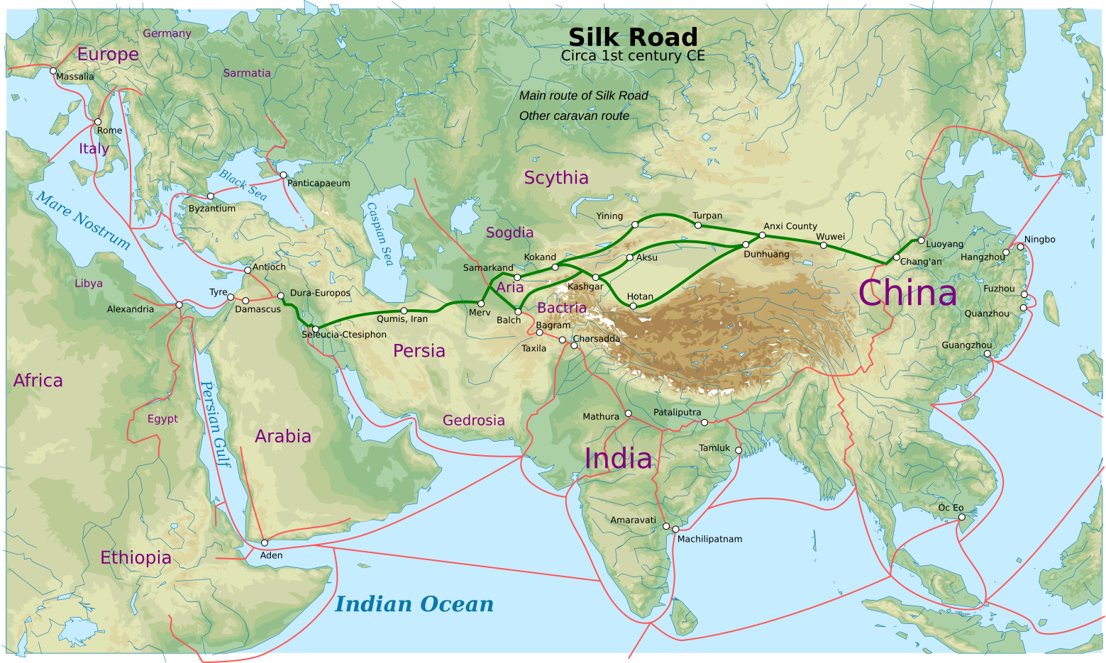
Figure 3.14:The Silk Road (Source: Wikimedia Commons)
Returning to the model, we allow for both initial supply of and final demand for the good at every node (although one or both could be zero). Let and be supply and demand at node respectively. Aggregate supply and demand over the network are assumed to be equal, so that
This can be understood as an equilibrium condition: prices have adjusted to equalize initial supply and final demand in aggregate. We assume throughout that the vectors and are nonnegative with at least one positive element.
Let be the amount of the good shipped from node to node for all . The minimum cost network flow problem is to minimize total shipping cost
subject to the restriction that and
The left hand side of (3.34) is total supply to node (initial supply plus inflow from other nodes), while the right hand side is total demand (final demand plus outflow to other nodes).
3.3.4.2Optimality
There are several ways to transform the network flow problem into a linear program. We follow the presentation in Bertsimas & Tsitsiklis (1997). We take to be the total number of edges and enumerate them (in any convenient way) as . Let’s say that leaves node if for some , and that enters node if for some . Then we define the node-edge incidence matrix by
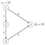
Figure 3.15:A simple network flow problem
Now, returning to the general case, we rearrange and into vectors and , where is the amount shipped along edge and is the cost. For example, if , then and . In addition, we set to be the vector in with -th element , which is net exogenous supply at node .
Equation (3.36) tells us that the -th row of give us the net outflow from node under the transport plan . Now, with , the minimum cost network flow problem can now be expressed as
This is a linear program in standard equality form, to which we can apply any linear programming solver. For Example 3.3.1, we run the following:
A = (( 1,  1,  0,  0),
     (-1,  0,  1,  0),
     ( 0,  0, -1,  1),
     ( 0, -1,  0, -1))

b = (10, 0, 0, -10)
c = (1, 4, 1, 1)

result = linprog(c, A_eq=A, b_eq=b, method='highs-ipm')
print(result.x)
The output is [10. 0. 10. 10.]. Recalling the order of the paths in (3.35), this means that the optimal transport plan is and , as our intuition suggests.
3.3.4.3Reduction to Optimal Transport
In Exercise 3.3.13, we saw how every optimal transport problem is a special kind of minimum cost network flow problem. There is a sense in which the converse is also true. In particular, we can use optimal transport methods to solve any network flow problem, provided that we first modify the network flow problem via an application of shortest paths.
To explain how this works, we take the abstract network flow problem described in Section 3.3.4.1, on the weighted digraph , with , initial supply vector and final demand vector . For the purposes of this section, we agree to call a node with a net supplier. A node with will be called a net consumer. Nodes with will be called trading stations.
The idea behind the reduction is to treat the net supplier nodes as source locations and the net consumer nodes as target locations in an optimal transport problem. The next step is to compute the shortest path (if there are multiple, pick any one) from each net supplier to each net consumer . Let denote this path, represented as a sequence of edges in . The cost of traversing is
Now the trading stations are eliminated and we solve the optimal transport problem with
the set of net suppliers,
the set of net consumers,
on ,
on , and
cost function as defined above.[5]
After we find the optimal transport plan , the network minimum cost flow along arbitrary edge is recovered by setting
Figure 3.16 illustrates the method. Trading station 3 is eliminated after the shortest paths are computed.
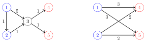
Figure 3.16:Reducing minimum cost optimal flow to optimal transport
3.4Chapter Notes
Our treatment of shortest paths can be understood as a simplified version of both the Bellman–Ford algorithm and Dijkstra’s algorithm, which are routinely used to solve large shortest path planning problems. Our approach is intended to emphasize recursive solution methods, which are valuable for analyzing a vast range of economic problems, from intertemporal modeling (see, e.g., Lucas & Stokey (1989) or Ljungqvist & Sargent (2018)) to production chains Kikuchi et al., 2021.
Betweenness centrality has been used to quantify the notion of “too connected to fail,” which gained attention after the 2007–2008 global financial crisis. For example, Huang et al. (2016) examine how betweenness centrality affects systemic risk. Betweenness centrality is used to examine liquidity shocks in the interbank markey by Chiu et al. (2020). Relatedly, Yun et al. (2019) propose a measure of “too central to fail” based on the PageRank algorithm.
For a more in-depth treatment of linear programming, we recommend the excellent textbooks by Bertsimas & Tsitsiklis (1997) and Matousek & Gärtner (2007). For bedtime reading, Cook (2011) provides an entertaining introduction to some of the main ideas and applications to network problems, including a review of computation.
While Section 3.2.1 provided a rather whimsical introduction to matching and assignment problems, such problems have great real world importance. Examples include assigning kidney donors to recipients, mothers to maternity wards, doctors to hospitals, students to schools, delivery drivers to orders and autonomous vehicles to riders.[6] A brief history of assignment, matching problems and combinatorial optimization can be found in Schrijver (2005). Greinecker & Kah (2021) study existence of stable matchings in a setting with many agents.
Villani (2008) and Vershik (2013) provide extensive historical background on the optimal transport problem. Vershik (2013) mentions some of the problems that Kantorovich faced, as a Soviet mathematician working in the time of Stalin and Khrushchev, given that his main duality theorem for optimal transport can be seen as a proof that competitive market equilibria attain the maximal transport plan.
In Section 3.3.2, we mentioned that Kantorovich’s work anticipated much of the later development of duality theory for arbitrary linear programs. In fact, according to Vershik (2013), Kantorovich anticipated much of the general theory of linear programming itself, including providing a version of the simplex algorithm later rediscovered and extended by Dantzig.
Optimal transport has a remarkably wide variety of applications, spread across economics, econometrics, finance, statistics, artificial intelligence, machine learning and other fields. Within economics, Galichon (2018) provides an excellent overview. Charpentier et al. (2019) and Fajgelbaum & Schaal (2020) consider optimal transport in spacial equilibria. Ocampo (2022) applies optimal transport measures to the study of tasks and occupations. Beiglböck et al. (2022) review some of the major milestones of modern finance theory and show their connections via optimal transport. Connections to machine learning are surveyed in Kolouri et al. (2017).
The computational theory of optimal transport is now a major field. A high quality exposition can be found in Peyré & Cuturi (2019). Blanchet et al. (2018) use computational optimal transport to solve for Cournot–Nash equilibria in mean-field type games.
Readers familiar with high performance computing techniques might suggest that the curse of dimensionality is no cause for concern for the matching problem, since the search algorithm be parallelized. Unfortunately, even the best parallelization methods cannot save the workstation from being vaporized by the sun with the calculation incomplete. The best-case scenario is that adding another execution thread doubles effective computations per second and hence halves execution time. However, even with such threads (an enormous number), the execution time would still be years.
For example, in image processing, two images might be regarded as close if the cost of transforming one into the other by altering individual pixels is small. Even now, in image processing and some branches of machine learning, one of the metrics over the set of probability distributions arising from optimal transport methods is referred to as “earth mover’s distance” in honor of the work of Monge.
The optimal transport problem continues to attract the interest of many brilliant mathematicians and economists, with two recent Fields Medals being awarded for work on optimal transport. The first was awarded to Cedric Villani in 2010, while the second was to Alessio Figalli in 2018. Note that the Field Medal is only awarded every four years (unlike the Nobel Prize, which is annual).
Our use of the Silk Road as an example of a network flow problem is not original. Galichon (2018) provides a highly readable treatment in the context of optimal transport.
If no path exists from to then we set . Such settings can be handled in linear programming solvers by adding capacity constraints. See, for example, Peyré & Cuturi (2019), Section 10.3.
The latter problem occurs in the field of Autonomous Mobility on Demand (AMoD). See, for example, Ascenzi & Palanza (2021) or Simonetto et al. (2019).
- Dantzig, G. B. (1951). Application of the simplex method to a transportation problem. Activity Analysis and Production and Allocation.
- Bertsimas, D., & Tsitsiklis, J. N. (1997). Introduction to linear optimization. Athena Scientific.
- Matousek, J., & Gärtner, B. (2007). Understanding and using linear programming. Springer Science & Business Media.
- Galichon, A. (2018). Optimal Transport Methods in Economics. Princeton University Press.
- Flamary, R., Courty, N., Gramfort, A., Alaya, M. Z., Boisbunon, A., Chambon, S., Chapel, L., Corenflos, A., Fatras, K., Fournier, N., Gautheron, L., Gayraud, N. T. H., Janati, H., Rakotomamonjy, A., Redko, I., Rolet, A., Schutz, A., Seguy, V., Sutherland, D. J., … Vayer, T. (2021). POT: Python Optimal Transport. Journal of Machine Learning Research, 22(78), 1–8. http://jmlr.org/papers/v22/20-451.html
- Lucas, R., & Stokey, N. (1989). Recursive methods in dynamic economics. Harvard University Press.
- Ljungqvist, L., & Sargent, T. J. (2018). Recursive macroeconomic theory (4th ed.). MIT press.
- Kikuchi, T., Nishimura, K., Stachurski, J., & Zhang, J. (2021). Coase meets Bellman: Dynamic programming for production networks. Journal of Economic Theory, 196, 105287.
- Huang, W.-Q., Zhuang, X.-T., Yao, S., & Uryasev, S. (2016). A financial network perspective of financial institutions’ systemic risk contributions. Physica A: Statistical Mechanics and Its Applications, 456, 183–196.
- Chiu, J., Eisenschmidt, J., & Monnet, C. (2020). Relationships in the interbank market. Review of Economic Dynamics, 35, 170–191.
- Yun, T.-S., Jeong, D., & Park, S. (2019). “Too central to fail” systemic risk measure using PageRank algorithm. Journal of Economic Behavior & Organization, 162, 251–272.
- Cook, W. J. (2011). In pursuit of the traveling salesman. Princeton University Press.
- Schrijver, A. (2005). On the history of combinatorial optimization (till 1960). Handbooks in Operations Research and Management Science, 12, 1–68.
- Greinecker, M., & Kah, C. (2021). Pairwise stable matching in large economies. Econometrica, 89(6), 2929–2974.
- Villani, C. (2008). Optimal transport: old and new (Vol. 338). Springer Science & Business Media.