Relations are the fundamental fabric of reality.
Michele Coscia
1.1Motivation¶
Alongside the exponential growth of computer networks over the last few decades, we have witnessed concurrent and equally rapid growth in a field called network science. Once computer networks brought network structure into clearer focus, scientists began to recognize networks almost everywhere, even in phenomena that had already received centuries of attention using other methods, and to apply network theory to organize and expand knowledge right throughout the sciences, in every field and discipline.
The set of possible examples is vast, and sources mentioning or treating hundreds of different applications of network methods and graph theory are listed in the reading notes at the end of the chapter. In computer science and machine learning alone, we see computational graphs, graphical networks, neural networks and deep learning. In operations research, network analysis focuses on minimum cost flow, traveling salesman, shortest path, and assignment problems. In biology, networks are a standard way to represent interactions between bioentities.
In this book, our interest lies in economic and social phenomena. Here, too, networks are pervasive. Important examples include financial networks, production networks, trade networks, transport networks and social networks. For example, social and information networks affect trends in sentiments and opinions, consumer decisions, and a range of peer effects. The topology of financial networks helps to determine relative fragility of the financial system, while the structure of production networks affects trade, innovation and the propagation of local shocks.
Figure 1.1–Figure 1.2 show two examples of trade networks. Figure 1.1 is called a Sankey diagram, which is a kind of figure used to represent flows. Oil flows from left to right. The countries on the left and below are the top 10 exporters of crude oil, while the countries on the right are the top 20 consumers. The figure relates to one of our core topics: optimal (and equilibrium) flows across networks. We treat optimal flows at length in Chapter 3.[1]
Figure 1.2 shows international trade in large commercial aircraft in 2019.[2] Node size is proportional to total exports and link width is proportional to exports to the target country. The US, France and Germany are revealed as major export hubs.
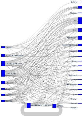
Figure 1.1:International trade in crude oil 2021
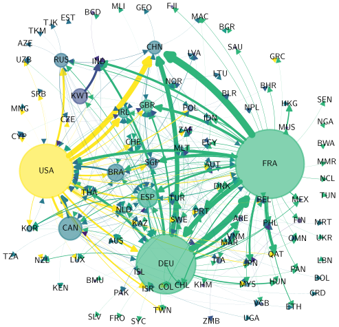
Figure 1.2:International trade in commercial aircraft during 2019
While some readers viewing Figure 1.1–Figure 1.2 might at first suspect that the network perspective adds little more than an attractive technique for visualizing data, it actually adds much more. For example, in Figure 1.2, node colors are based on a ranking of “importance” in the network called eigenvector centrality, which we introduce in Section 1.4.3.4. Such rankings and centrality measures are an active area of research among network scientists. Eigenvector and other forms of centrality feature throughout the text. For example, we will see that these concepts are closely connected to—and shed new light on—fundamental ideas first developed many years ago by researchers in the field of input-output economics.
In addition, in production networks, it turns out that the nature of shock propagation is heavily dependent on the underlying structure of the network. For example, for a few highly connected nodes, shocks occurring within one firm or sector can have an outsized influence on aggregate-level fluctuations. Economists are currently racing to understand these relationships, their interactions with various centrality measures, and other closely related phenomena.
To understand this line of work, as well as other applications of network methods to economics and finance, some technical foundations are required. For example, to define eigenvector centrality, we need to be familiar with eigenvectors, spectral decompositions and the Perron–Frobenius theorem. To work with Katz centrality, which also features regularly in network science and economics, we require a sound understanding of the Neumann series lemma. The Perron–Frobenius theorem and the Neumann series lemma form much of the technical foundation of this textbook. We review them in detail in Section 1.2 and develop extensions throughout remaining chapters.
One reason that analysis of networks is challenging is high-dimensionality. To see why, consider implementing a model with economic agents. This requires times more data than one representative agent in a setting where agents are atomistic or coordinated by a fixed number of prices. For example, Carvalho & Grassi (2019) model the dynamics of firms, all of which need to be tracked when running a simulation. However, if we wish to model interactions between each pair (supply linkages, liabilities, etc.), then, absent sparsity conditions, the data processing requirement grows like .[3] In the Carvalho & Grassi (2019) example, is , which is very large even for modern computers. One lesson is that network models can be hard to solve, even with powerful computers, unless we think carefully about algorithms.
In general, to obtain a good grasp on the workings of economic networks, we will need computational skills plus a firm understanding of linear algebra, probability and a field of discrete mathematics called graph theory. The rest of this chapter provides relevant background in these topics. Before tackling this background, we recommend that readers skim the list of common symbols, as well the mathematical topics in the appendix, which start. (The appendix is not intended for sequential reading, but rather as a source of definitions and fundamental results to be drawn on in what follows.)
1.2Spectral Theory¶
In this section we review some linear algebra needed for the study of graphs and networks. Highlights include the spectral decomposition of diagonalizable matrices, the Neumann series lemma, and the theorem of Perron and Frobenius.
1.2.1Eigendecompositions¶
Our first task is to cover spectral decompositions and the spectral theorem. We begin with a brief review of eigenvalues and their properties. (If you are not familiar with eigenvalues and eigenvectors, please consult an elementary treatment first. See, for example, Cohen (2021).)
1.2.1.1Eigenvalues¶
Fix in . A scalar is called an eigenvalue of if there exists a nonzero complex vector such that . A vector satisfying this equality is called an eigenvector corresponding to the eigenvalue . (Notice that eigenvalues and eigenvectors are allowed to be complex, even though we restrict elements of to be real.) The set of all eigenvalues of is called the spectrum of and written as . As we show below, has at most distinct eigenvalues.
In Julia, we can check for the eigenvalues of a given square matrix via eigvals(A). Here is one example
using LinearAlgebra
A = [0 -1;
1 0]
eigenvals = eigvals(A) Running this code in a Jupyter cell (with Julia kernel) or Julia REPL produces
2-element Vector{ComplexF64}:
0.0 - 1.0im
0.0 + 1.0imHere im stands for , the imaginary unit (i.e., ).
If and is an eigenvector for , then is called an eigenpair.
It can be shown that is a polynomial of degree .[4] This polynomial is called the characteristic polynomial of . By the Fundamental Theorem of Algebra, there are roots (i.e., solutions in to the equation ), although some may be repeated as in the complete factorization of . By Lemma 1.2.1,
each of these roots is an eigenvalue, and
no other eigenvalues exist besides these roots.
If appears times in the factorization of the polynomial , then is said to have algebraic multiplicity . An eigenvalue with algebraic multiplicity one is called simple. A simple eigenvalue has the property that its eigenvector is unique up to a scalar multiple, in the sense of Exercise 1.2.2. In other words, the linear span of (called the eigenspace of ) is one-dimensional.
1.2.1.2The Eigendecomposition¶
What are the easiest matrices to work with? An obvious answer to this question is: the diagonal matrices. For example, when with ,
the linear system reduces to completely independent scalar equations,
the -th power is just , and
the inverse is just , assuming all ’s are nonzero.
While most matrices are not diagonal, there is a way that “almost any” matrix can be viewed as a diagonal matrix, after translation of the usual coordinates in via an alternative basis. This can be extremely useful. The key ideas are described below.
is called diagonalizable if
We allow both and to contain complex values. The representation is called the eigendecomposition or the spectral decomposition of .
One way to think about diagonalization is in terms of maps, as in

Either we can map directly with or, alternatively, we can shift to via , apply the diagonal matrix , and then shift back to via .
The equality can also be written as . Decomposed across column vectors, this equation says that each column of is an eigenvector of and each element along the principal diagonal of is an eigenvalue.
When does diagonalizability hold?
While diagonalizability is not universal, the set of matrices in that fail to be diagonalizable has “Lebesgue measure zero” in . (Loosely speaking, only special or carefully constructed examples will fail to be diagonalizable.) The next results provide conditions for the property.
This result is intuitive: for to hold we need to be invertible, which requires that its columns are linearly independent. Since is -dimensional, this means that the columns form a basis of .
There is another way that we can establish diagonalizability, based on symmetry. Symmetry also lends the diagonalization certain properties that turn out to be very useful in applications. We are referring to the following celebrated theorem.
Since, for the orthonormal matrix , we have (see Lemma 6.1.15), one consequence of the spectral theorem is that is diagonalizable. For obvious reasons, we often say that is orthogonally diagonalizable.
1.2.1.3Worker Dynamics¶
Let’s study a small application of the eigendecomposition. Suppose that, each month, workers are hired at rate and fired at rate . Their two states are unemployment (state 1) and employment (state 2). Figure 1.3 shows the transition probabilities for a given worker in each of these two states.
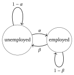
Figure 1.3:Worker transition dynamics
We translate these dynamics into the matrix
Row 1 of gives probabilities for unemployment and employment respectively when currently unemployed.
Row 2 of gives probabilities for unemployment and employment respectively when currently employed.
Below we demonstrate that the -th power of provides -step transition probabilities for workers. Anticipating this discussion, we now seek an expression for at arbitrary . This problem is simplified if we use diagonalization.
1.2.1.4Left Eigenvectors¶
A vector is called a left eigenvector of if is an eigenvector of . In other words, is nonzero and there exists a such that . We can alternatively write the expression as , which is where the name “left” eigenvector originates.
Left eigenvectors will play important roles in what follows, including that of stochastic steady states for dynamic models under a Markov assumption. To help distinguish between ordinary and left eigenvectors, we will at times call (ordinary) eigenvectors of right eigenvectors of .
If is diagonalizable, then so is . To show this, let with . We know from earlier discussion that the columns of are the (right) eigenvectors of .
The results of the last exercise show that, when , the columns of coincide with the left eigenvectors of . (Why?) Equivalently, where is the matrix with -th column equal to the -th left eigenvector of .
1.2.1.5Similar Matrices¶
Diagonalizability is a special case of a more general concept: is called similar to if there exists an invertible matrix such that . In this terminology, is diagonalizable if and only if it is similar to a diagonal matrix.
The last result is a generalization of (1.1). When is large, calculating the powers can be computationally expensive or infeasible. If, however, is similar to some simpler matrix , then we can take powers of instead, and then transition back to using the similarity relation.[5]
1.2.2The Neumann Series Lemma¶
Most high school students learn that, if is a number with , then
This geometric series representation extends to matrices: If is a matrix satisfying a certain condition, then (1.6) holds, in the sense that . (Here is the identity matrix.) But what is the “certain condition” that we need to place on , which generalizes the concept to matrices? The answer to this question involves the “spectral radius” of a matrix, which we now describe.
1.2.2.1Spectral Radius¶
Fix . With indicating the modulus of a complex number , the spectral radius of is defined as
Within economics, the spectral radius has important applications in dynamics, asset pricing, and numerous other fields. As we will see, the same concept also plays a key role in network analysis.
After executing
import numpy as npThe following Python code computes the spectral radius of a square matrix :
def spec_rad(M):
return np.max(np.abs(np.linalg.eigvals(M))) 1.2.2.2Geometric Series¶
We can now return to the matrix extension of (1.6) and state a formal result.
The sum is called the power series representation of . Convergence of the matrix series is understood as element-by-element convergence.
A full proof of Theorem 1.2.5 can be found in Cheney (2013) and many other sources. The core idea is simple: if then . Reorganizing gives , which is equivalent to (1.8). The main technical issue is showing that the power series converges. The full proof shows that this always holds when .
1.2.3The Perron–Frobenius Theorem¶
In this section we state and discuss a suprisingly far reaching theorem due to Oskar Perron and Ferdinand Frobenius, which has applications in network theory, machine learning, asset pricing, Markov dynamics, nonlinear dynamics, input-output analysis and many other fields. In essence, the theorem provides additional information about eigenvalues and eigenvectors when the matrix in question is positive in some sense.
1.2.3.1Order in Matrix Space¶
We require some definitions. In what follows, for , we write
if all elements of are nonnegative and
if all elements of are strictly positive.
It’s easy to imagine how nonnegativity and positivity are important notions for matrices, just as they are for numbers. However, strict positivity of every element of a matrix is hard to satisfy, especially for a large matrix. As a result, mathematicians routinely use two notions of “predominantly strictly positive,” which sometimes provide sufficient positivity for the theorems that we need.
Regarding these two notions, for , we say that is
irreducible if and
primitive if there exists an such that .
Evidently, for we have
A nonnegative matrix is called reducible if it fails to be irreducible.
In addition to the above notation, for , we also write
if and if ,
if , etc.
The partial order discussed in Exercise 1.2.21 is usually called the pointwise partial order on . Analogous notation and terminology are used for vectors.
The following exercise shows that nonnegative matrices are order-preserving maps (see Section 6.1.2.3) on vector space under the pointwise partial order—a fact we shall exploit many times.
1.2.3.2Statement of the Theorem¶
Let be in . In general, is not an eigenvalue of . For example,
But is always an eigenvalue when . This is just one implication of the following famous theorem.
The fact that is simple under irreducibility means that its eigenvectors are unique up to scalar multiples. We will exploit this property in several important uniqueness proofs.
In the present context, is called the dominant eigenvalue or Perron root of , while and are called the dominant left and right eigenvectors of , respectively.
Why do we use the word “dominant” here? To help illustrate, let us suppose that is primitive and fix any . Consider what happens to the point as grows. By (1.11) we have for large , where . In other words, asymptotically, the sequence is just scalar multiples of , growing at rate . Thus, dominates other eigenvalues in controlling the growth rate of , while dominates other eigenvectors in controlling the direction of growth.
1.2.3.3Worker Dynamics II¶
We omit the full proof of Theorem 1.2.6, which is quite long and can be found in Meyer (2000), Seneta (2006) or Meyer-Nieberg (2012).[6] Instead, to build intuition, let us prove the theorem in a rather simple special case.
The special case we will consider is the class of matrices
This example is drawn from the study of worker dynamics in Section 1.2.1.3.
You might recall from Section 1.2.1.3 that and . Clearly , so is an eigenvalue, as claimed by the first part of the Perron–Frobenius theorem.
From now on we assume that , which just means that we are excluding the identity matrix in order to avoid some tedious qualifying remarks.
The two right eigenvectors () and two left eigenvectors () are, respectively,
1.2.3.4Bounding the Spectral Radius¶
Using the Perron–Frobenius theorem, we can provide useful bounds on the spectral radius of a nonnegative matrix. In what follows, fix and set
the -th row sum of and
the -th column sum of .
1.3Probability¶
Next we review some elements of probability that will be required for analysis of networks.
1.3.1Discrete Probability¶
We first introduce probability models on finite sets and then consider sampling methods and stochastic matrices.
1.3.1.1Probability on Finite Sets¶
Throughout this text, if is a finite set, then we set
and call the set of distributions on . We say that a random variable taking values in has distribution and write if
A distribution can also be understood as a vector (see Lemma 6.1.2 in Section 6.1.1.3). As a result, can be viewed as a subset of . Figure 1.4 provides a visualization when . Each is identified by the point in .
More generally, if , then can be identified with the unit simplex in , which is the set of all -vectors that are nonnegative and sum to one.
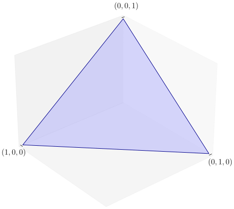
Figure 1.4:If , then is the unit simplex in
Throughout, given , we use the symbol to represent the element of that puts all mass on . In other words, for all . In Figure 1.4, each is a vertex of the unit simplex.
We frequently make use of the law of total probability, which states that, for a random variable on and arbitrary ,
where is a partition of (i.e., finite collection of disjoint subsets of such that their union equals ).
1.3.1.2Inverse Transform Sampling¶
Let be a finite set. Suppose we have the ability to generate random variables that are uniformly distributed on . We now want to generate random draws from that are distributed according to arbitrary .
Let be uniformly distributed on , so that, for any , we have , which is the length of the interval .[7] Our problem will be solved if we can create a function from to such that has distribution . One technique is as follows. First we divide the unit interval into disjoint subintervals, one for each . The interval corresponding to is denoted and is chosen to have length . More specifically, when , we take
You can easily confirm that the length of is for all .
Now consider the function defined by
where is one when and zero otherwise. It turns out that has the distribution we desire.
The last exercise tells us that that the law of large numbers holds in this setting, since, under this law, we expect that
with probability one as . In view of Exercise 1.3.3, the right hand side equals .
1.3.1.3Stochastic Matrices¶
A matrix is called a stochastic matrix if
In other words, is nonnegative and has unit row sums.
We will see many applications of stochastic matrices in this text. Often the applications are probabilistic, where each row of is interpreted as a distribution over a finite set.
The vector in part (iii) of Exercise 1.3.7 is called the PageRank vector by some authors, due to its prominence in Google’s PageRank algorithm. We will call it a stationary distribution instead.[8] Stationary distributions play a key role in the theory of Markov chains, to be treated in Section 4.1. Ranking methods are discussed again in Section 1.4.3. PageRank is treated in more detail in Section 4.2.3.3.
1.3.2Power Laws¶
Next we discuss distributions on the (non-discrete) sets and . We are particularly interested in a certain class of distributions that are apparently non-standard and yet appear with surprising regularity in economics, social science, and the study of networks. We refer to the distributions that are said to obey a “power law.”
In what follows, given a real-valued random variable , the function
is called the cumulative distribution function (CDF) of . The counter CDF (CCDF) of is the function .
A useful property that holds for any nonnegative random variable and is the identity
See, for example, Çınlar (2011), p. 63.
1.3.2.1Heavy Tails¶
Recall that a random variable on is said to be normally distributed with mean and variance , and we write , if has density
One notable feature of the normal density is that the tails of the density approach zero quickly. For example, goes to zero like as , which is extremely fast.
A random variable on is called exponentially distributed and we write if, for some , has density
The tails of the exponential density go to zero like as , which is also relatively fast.
When a distribution is relatively light-tailed, in the sense that its tails go to zero quickly, draws rarely deviate more than a few standard deviations from the mean. In the case of a normal random variable, the probability of observing a draw more than 3 standard deviations above the mean is around 0.0014. For 6 standard deviations, the probability falls to .
In contrast, for some distributions, “extreme” outcomes occur relatively frequently. The left panel of Figure 1.5 helps to illustrate by simulating 1,000 independent draws from Student’s t-distribution, with degrees of freedom. For comparison, the right subfigure shows an equal number of independent draws from the distribution. The Student’s t draws reveal tight clustering around zero combined with a few large deviations.
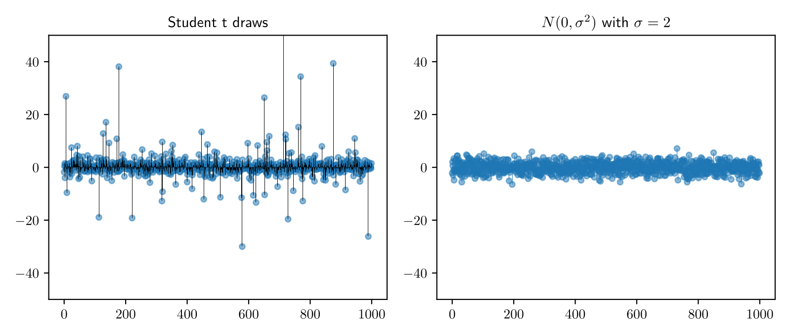
Figure 1.5:Independent draws from Student’s t- and normal distributions
Formally, a random variable on is called light-tailed if its moment generating function
is finite for at least one . Otherwise is called heavy-tailed.[9]
For any random variable and any , the (possibly infinite) expectation called the -th moment of .
Together with Lemma 1.3.1, Exercise 1.3.8 shows that existence of an infinite moment is a sufficient but not necessary condition for heavy tails.
1.3.2.2Pareto Tails¶
Given , a nonnegative random variable is said to have a Pareto tail with tail index if there exists a such that
In other words, the CCDF of satisfies
If has a Pareto tail for some , then is also said to obey a power law.
Regarding Example 1.3.3, note that the converse is not true: Pareto-tailed random variables are not necessarily Pareto distributed, since the Pareto tail property only restricts the far right hand tail.
From Exercise 1.3.9 and Lemma 1.3.1, we see that every Pareto-tailed random variable is heavy-tailed. The converse is not true, since the Pareto tail property (1.16) is very specific. Despite this, it turns out that many heavy-tailed distributions encountered in the study of networks are, in fact, Pareto-tailed.
1.3.2.3Empirical Power Law Plots¶
When the Pareto tail property holds, the CCDF satisfies for large . In other words, is eventually log linear. Figure 1.6 illustrates this using a Pareto distribution. For comparison, the CCDF of an exponential distribution is also shown.
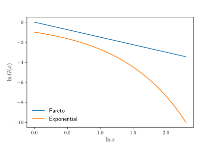
Figure 1.6:CCDF plots for the Pareto and exponential distributions
If we replace the CCDF with its empirical counterpart—which returns, for each , the fraction of the sample with values greater than —we should also obtain an approximation to a straight line under the Pareto tail assumption.
For example, consider the cross-sectional distribution of firm sizes. While the precise nature of this distribution depends on the measure of firm size, the sample of firms and other factors, the typical picture is one of extreme heavy tails. As an illustration, Figure 1.7 shows an empirical CCDF log-log plot for market values of the largest 500 firms in the Forbes Global 2000 list, as of March 2021. The slope estimate and data distribution are consistent with a Pareto tail and infinite population variance.
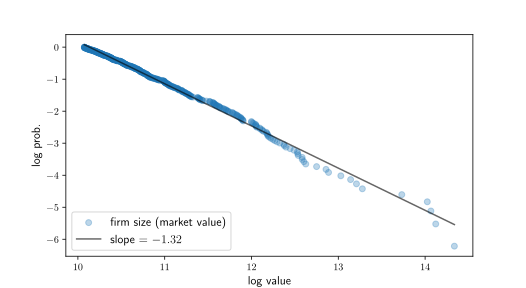
Figure 1.7:Empirical CCDF plots for largest firms (Forbes)
1.3.2.4Discrete Power Laws¶
Let be a random variable with the Pareto distribution, as described in Example 1.3.3. The density of this random variable on the set is with and . The next exercise extends this idea.
The discrete analog of (1.19) is a distribution on the positive integers with
for large . In the special case where this equality holds for all , and is chosen so that , we obtain the zeta distribution.[10]
In general, when we see a probability mass function with the specification (1.20) for large , we can identify this with a Pareto tail, with tail index . Figure 1.8 illustrates with .
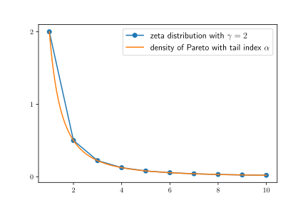
Figure 1.8:Zeta and Pareto distributions
1.4Graph Theory¶
Graph theory is a major branch of discrete mathematics. It plays an essential role in this text because it forms the foundations of network analysis. This section provides a concise introduction to graph theory suitable for our purposes.[11]
Graph theory has another closely related use: many economic models are stochastic and dynamic, which means that they specify states of the world and rates of transition between them. One of the most natural ways to conceptualize these notions is to view states as vertices in a graph and transition rates as relationships between them.
We begin with definitions and fundamental concepts. We focus on directed graphs, where there is a natural asymmetry in relationships (bank lends money to bank , firm supplies goods to firm , etc.). This costs no generality, since undirected graphs (where relationships are symmetric two-way connections) can be recovered by insisting on symmetry (i.e., existence of a connection from to implies existence of a connection from to ).
1.4.1Unweighted Directed Graphs¶
We begin with unweighted directed graphs and examine standard properties, such as connectedness and aperiodicity.
1.4.1.1Definition and Examples¶
A directed graph or digraph is a pair , where
is a finite nonempty set and
is a collection of ordered pairs called edges.
Elements of are called the vertices or nodes of . Intuitively and visually, an edge is understood as an arrow from vertex to vertex .
Two graphs are given in Figure 1.9–Figure 1.10. Each graph has three vertices. In these cases, the arrows (edges) could be thought of as representing positive possibility of transition over a given unit of time.
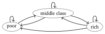
Figure 1.9:A digraph of classes
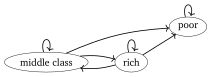
Figure 1.10:An alternative edge list
For a given edge , the vertex is called the tail of the edge, while is called the head. Also, is called a direct predecessor of and is called a direct successor of . For , we use the following notation:
the set of all direct predecessors of
the set of all direct successors of
Also, the in-degree and out-degree of are defined by
the and
the respectively.
If and , then is called a source. If either or , then is called a sink. For example, in Figure 1.10, “poor” is a sink with an in-degree of 3.
1.4.1.2Digraphs in Networkx¶
Both Python and Julia provide valuable interfaces to numerical computing with graphs. Of these libraries, the Python package Networkx is probably the most mature and fully developed. It provides a convenient data structure for representing digraphs and implements many common routines for analyzing them. To import it into Python we run
import networkx as nxIn all of the code snippets shown below, we assume readers have executed this import statement, as well as
import numpy as np
import matplotlib.pyplot as pltAs an example, let us create the digraph in Figure 1.10, which we denote henceforth by . To do so, we first create an empty DiGraph object:
G_p = nx.DiGraph() Next we populate it with nodes and edges. To do this we write down a list of all edges, with poor represented by p and so on:
edge_list = [
('p', 'p'),
('m', 'p'), ('m', 'm'), ('m', 'r'),
('r', 'p'), ('r', 'm'), ('r', 'r')
]Finally, we add the edges to our DiGraph object:
for e in edge_list:
u, v = e
G_p.add_edge(u, v)Adding the edges automatically adds the nodes, so G_p is now a correct representation of . For our small digraph we can verify this by plotting the graph via Networkx with the following code:
fig, ax = plt.subplots()
nx.draw_spring(G_p, ax=ax, node_size=500, with_labels=True,
font_weight='bold', arrows=True, alpha=0.8,
connectionstyle='arc3,rad=0.25', arrowsize=20)
plt.show()This code produces Figure 1.11, which matches the original digraph in Figure 1.10.
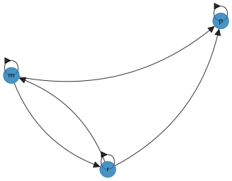
Figure 1.11:Networkx digraph plot
DiGraph objects have methods that calculate in-degree and out-degree of vertices. For example,
G_p.in_degree('p')prints 3.
1.4.1.3Communication¶
Next we study communication and connectedness, which have important implications for production, financial, transportation and other networks, as well as for dynamic properties of Markov chains.
A directed walk from vertex to vertex of a digraph is a finite sequence of vertices, starting with and ending with , such that any consecutive pair in the sequence is an edge of . A directed path from to is a directed walk from to such that all vertices in the path are distinct. For example, in Figure 1.12, is a directed walk from to but not a directed path, while is both a directed path and a directed walk from to .
As is standard, the length of a directed walk (or path) counts the number of edges rather than vertices. For example, the directed path from to in Figure 1.12 is said to have length 2.
Vertex is called accessible (or reachable) from vertex , and we write , if either or there exists a directed path from to . A set is called absorbing for the directed graph if no element of is accessible from .
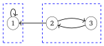
Figure 1.12:Strongly connected components of a digraph (rectangles)
Two vertices and are said to communicate if and .
Since communication is an equivalence relation, it induces a partition of into a finite collection of equivalence classes. Within each of these classes, all elements communicate. These classes are called strongly connected components. The graph itself is called strongly connected if there is only one such component; that is, is accessible from for any pair . This corresponds to the idea that any node can be reached from any other.
Networkx can be used to test for communication and strong connectedness, as well as to compute strongly connected components. For example, applied to the digraph in Figure 1.12, the code
G = nx.DiGraph()
G.add_edge(1, 1)
G.add_edge(2, 1)
G.add_edge(2, 3)
G.add_edge(3, 2)
list(nx.strongly_connected_components(G)) prints [{1}, {2, 3}].
1.4.1.4Aperiodicity¶
A cycle of a directed graph is a directed walk in such that (i) the first and last vertices are equal and (ii) no other vertex is repeated. The graph is called a directed acyclic graph if it contains no cycles. The graph is called periodic if it contains at least one cycle and, moreover, there exists a such that the length of every cycle is a multiple of . The graph is called aperiodic if it is not periodic.

Figure 1.13:A periodic digraph
An obvious sufficient condition for aperiodicity is existence of even one self-loop. The digraphs in Figure 1.9–Figure 1.12 are aperiodic for this reason.
The next result provides an easy way to understand aperiodicity for connected graphs. Proofs can be found in Häggström (2002) and Norris (1998).
It is common to call a vertex satisfying the condition in Lemma 1.4.1 aperiodic. With this terminology, Lemma 1.4.1 states that a strongly connected digraph is aperiodic if and only if every vertex is aperiodic.
Networkx can be used to check for aperiodicity of vertices or graphs. For example, if G is a DiGraph object, then nx.is_aperiodic(G) returns True or False depending on aperiodicity of G.
1.4.1.5Adjacency Matrices¶
There is a simple map between edges of a graph with fixed vertices and a binary matrix called an adjacency matrix. The benefit of viewing connections through adjacency matrices is that they bring the power of linear algebra to the analysis of digraphs. We illustrate this briefly here and extensively in Section 1.4.2.
If is a digraph with , then the adjacency matrix corresponding to is defined by[12]
For example, with poor, middle, rich mapped to , the adjacency matrix corresponding to the digraph in Figure 1.10 is
An adjacency matrix provides us with enough information to recover the edges of a graph. More generally, given a set of vertices , an matrix with binary entries generates a digraph with vertices and edges
The adjacency matrix of this graph is .
Like Networkx, the Python library quantecon provides a graph object that supplies certain graph-theoretic algorithms. In the case of QuantEcon’s DiGraph object, algorithms are implemented by interfacing with routines in SciPy and an instance is created by supplying an adjacency matrix. For example, to construct a digraph corresponding to Figure 1.10 we use the corresponding adjacency matrix (1.22):
import quantecon as qe
import numpy as np
A = ((1, 0, 0),
(1, 1, 1,),
(1, 1, 1))
A = np.array(A) # Convert to NumPy array
G = qe.DiGraph(A)Let’s print the set of strongly connected components, as a list of NumPy arrays:
G.strongly_connected_components The output is [array([0]), array([1, 2])].
1.4.2Weighted Digraphs¶
Early quantitative work on networks tended to focus on unweighted digraphs, where the existence or absence of an edge is treated as sufficient information (e.g., following or not following on social media, existence or absence of a road connecting two towns). However, for some networks, this binary measure is less significant than the size or strength of the connection.
As one illustration, consider Figure 1.14, which shows flows of funds (i.e., loans) between private banks, grouped by country of origin. An arrow from Japan to the US, say, indicates aggregate claims held by Japanese banks on all US-registered banks, as collected by the Bank of International Settlements (BIS). The size of each node in the figure is increasing in the total foreign claims of all other nodes on this node. The widths of the arrows are proportional to the foreign claims they represent.[13] The country codes are given in Table Table 1.1.
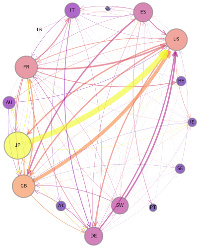
Figure 1.14:International private credit flows by country
Table 1.1:Codes for the 16-country financial network
AU | Australia | DE | Germany | CL | Chile | ES | Spain |
PT | Portugal | FR | France | TR | Turkey | GB | United Kingdom |
US | United States | IE | Ireland | AT | Austria | IT | Italy |
BE | Belgium | JP | Japan | SW | Switzerland | SE | Sweden |
In this network, an edge exists for almost every choice of and (i.e., almost every country in the network).[14] Hence existence of an edge is not particularly informative. To understand the network, we need to record not just the existence or absence of a credit flow, but also the size of the flow. The correct data structure for recording this information is a “weighted directed graph,” or “weighted digraph.” In this section we define this object and investigate its properties.
1.4.2.1Definitions¶
A weighted digraph is a triple such that is a digraph and is a function from to , called the weight function.
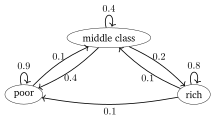
Figure 1.15:A weighted digraph
The definitions of accessibility, communication, periodicity and connectedness extend to any weighted digraph by applying them to . For example, is called strongly connected if is strongly connected. The weighted digraph in Figure 1.15 is strongly connected.
1.4.2.2Adjacency Matrices of Weighted Digraphs¶
In Section 1.4.1.5 we discussed adjacency matrices of unweighted digraphs. The adjacency matrix of a weighted digraph with vertices is the matrix
Clearly, once the vertices in are enumerated, the weight function and adjacency matrix provide the same information. We often work with the latter, since it facilitates computations.
In QuantEcon’s DiGraph implementation, weights are recorded via the keyword weighted:
A = ((0.9, 0.1, 0.0),
(0.4, 0.4, 0.2),
(0.1, 0.1, 0.8))
A = np.array(A)
G = qe.DiGraph(A, weighted=True) # Store weightsOne of the key points to remember about adjacency matrices is that taking the transpose “reverses all the arrows” in the associated digraph.
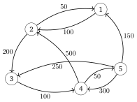
Figure 1.16:A network of credit flows across institutions
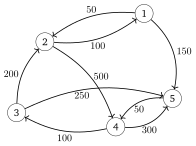
Figure 1.17:The transpose: a network of liabilities
It is not difficult to see that each nonnegative matrix can be viewed as the adjacency matrix of a weighted digraph with vertices equal to . The weighted digraph in question is formed by setting
We call the weighted digraph induced by .
The next exercise helps to reinforce the point that transposes reverse the edges.
1.4.2.3Application: Quadratic Network Games¶
Acemoglu et al. (2016) and Zenou (2016) consider quadratic games with agents where agent seeks to maximize
Here , is a symmetric matrix with for all , is a parameter and is a random vector. (This is the set up for the quadratic game in §21.2.1 of Acemoglu et al. (2016).) The -th agent takes the decisions as given for all when maximizing (1.26).
In this context, is understood as the adjacency matrix of a graph with vertices , where each vertex is one agent. We can reconstruct the weighted digraph by setting and letting be all pairs in with . The weights identify some form of relationship between the agents, such as influence or friendship.
The network game described in this section has many interesting applications, including social networks, crime networks and peer networks. References are provided in Section 1.5.
1.4.2.4Properties¶
In this section, we examine some of the fundamental properties of and relationships among digraphs, weight functions and adjacency matrices. Throughout this section, without loss of generality, we consider a weighted digraph with .
As an additional convention, if is an adjacency matrix, and is the -th power of , then we write for a typical element of . With this notation, we observe that, since , the rules of matrix multiplication imply
( is the identity.) The next proposition explains the significance of the powers.
In this context, the next result is fundamental.
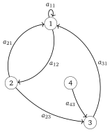
Figure 1.18:Failure of strong connectivity
We will find that the property of being primitive is valuable for analysis. (The Perron–Frobenius Theorem hints at this.) What do we need to add to strong connectedness to obtain primitiveness?
1.4.3Network Centrality¶
When studying networks of all varieties, a recurring topic is the relative “centrality” or “importance” of different nodes. One classic application is the ranking of web pages by search engines. Here are some examples related to economics:
In which industry will one dollar of additional demand have the most impact on aggregate production, once we take into account all the backward linkages? In which sector will a rise in productivity have the largest effect on national output?
A negative shock endangers the solvency of the entire banking sector. Which institutions should the government rescue, if any?
In the network games considered in Section 1.4.2.3, the Nash equilibrium is . Players’ actions are dependent on the topology of the network, as encoded in . A common finding is that the level of activity or effort exerted by an agent (e.g., severity of criminal activity by a participant in a criminal network) can be predicted from their “centrality” within the network.
In this section we review essential concepts related to network centrality.[15]
1.4.3.1Centrality Measures¶
Let be the set of weighted digraphs. A centrality measure associates to each in a vector , where the -th element of is interpreted as the centrality (or rank) of vertex . In most cases is nonnegative. In what follows, to simplify notation, we take .
(Unfortunately, the definitions and terminology associated with even the most common centrality measures vary widely across the applied literature. Our convention is to follow the mathematicians, rather than the physicists. For example, our terminology is consistent with Benzi & Klymko (2015).)
1.4.3.2Authorities vs Hubs¶
Search engine designers recognize that web pages can be important in two different ways. Some pages have high hub centrality, meaning that they link to valuable sources of information (e.g., news aggregation sites) . Other pages have high authority centrality, meaning that they contain valuable information, as indicated by the number and significance of incoming links (e.g., websites of respected news organizations). Figure 1.19 helps to visualize the difference.
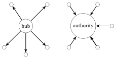
Figure 1.19:Hub vs authority
Similar ideas can and have been applied to economic networks (often using different terminology). For example, in production networks we study below, high hub centrality is related to upstreamness: such sectors tend to supply intermediate goods to many important industries. Conversely, a high authority ranking will coincide with downstreamness.
In what follows we discuss both hub-based and authority-based centrality measures, providing definitions and illustrating the relationship between them.
1.4.3.3Degree Centrality¶
Two of the most elementary measures of “importance” of a vertex in a given digraph are its in-degree and out-degree. Both of these provide a centrality measure. In-degree centrality is defined as the vector . Out-degree centrality is defined as . If is expressed as a Networkx DiGraph called G (see, e.g., Section 1.4.1.2), then can be calculated via
iG = [G.in_degree(v) for v in G.nodes()] This method is relatively slow when is a large digraph. Since vectorized operations are generally faster, let’s look at an alternative method using operations on arrays.
To illustrate the method, recall the network of financial institutions in Figure 1.16. We can compute the in-degree and out-degree centrality measures by first converting the adjacency matrix, which is shown in (1.24), to a binary matrix that corresponds to the adjacency matrix of the same network viewed as an unweighted graph:
Now if and only if points to . The out-degree and in-degree centrality measures can be computed as
respectively. That is, summing the rows of gives the out-degree centrality measure, while summing the columns gives the in-degree measure.
The out-degree centrality measure is a hub-based ranking, while the vector of in-degrees is an authority-based ranking. For the financial network in Figure 1.16, a high out-degree for a given institution means that it lends to many other institutions. A high in-degree indicates that many institutions lend to it.
Notice that, to switch from a hub-based ranking to an authority-based ranking, we need only transpose the (binary) adjacency matrix . We will see that the same is true for other centrality measures. This is intuitive, since transposing the adjacency matrices reverses the direction of the edges (Exercise 1.4.4).
For a weighted digraph with adjacency matrix , the weighted out-degree centrality and weighted in-degree centrality measures are defined as
respectively, by analogy with (1.29). We present some intuition for these measures in applications below.
Unfortunately, while in- and out-degree measures of centrality are simple to calculate, they are not always informative. As an example, consider again the international credit network shown in Figure 1.14. There, an edge exists between almost every node, so the in- or out-degree based centrality ranking fails to effectively separate the countries. This can be seen in the out-degree ranking of countries corresponding to that network in the top left panel of Figure 1.20, and in the in-degree ranking in the top right.
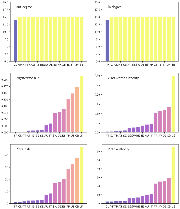
Figure 1.20:Centrality measures for the credit network
There are other limitations of degree-based centrality rankings. For example, suppose web page A has many inbound links, while page B has fewer. Even though page A dominates in terms of in-degree, it might be less important than web page B to, say, a potential advertiser, when the links into B are from more heavily trafficked pages. Thinking about this point suggests that importance can be recursive: the importance of a given node depends on the importance of other nodes that link to it. The next set of centrality measures we turn to has this recursive property.
1.4.3.4Eigenvector Centrality¶
Let be a weighted digraph with adjacency matrix . Recalling that is the spectral radius of , the hub-based eigenvector centrality of is defined as the that solves
Element-by-element, this is
Note the recursive nature of the definition: the centrality obtained by vertex is proportional to a sum of the centrality of all vertices, weighted by the “rates of flow” from into these vertices. A vertex is highly ranked if (a) there are many edges leaving , (b) these edges have large weights, and (c) the edges point to other highly ranked vertices.
When we study demand shocks in Section 2.1.3, we will provide a more concrete interpretation of eigenvector centrality. We will see that, in production networks, sectors with high hub-based eigenvector centrality are important suppliers. In particular, they are activated by a wide array of demand shocks once orders flow backwards through the network.
As the name suggests, hub-based eigenvector centrality is a measure of hub centrality: vertices are awarded high rankings when they point to important vertices. The next two exercises help to reinforce this point.
To compute eigenvector centrality when the adjacency matrix is primitive, we can employ the Perron–Frobenius Theorem, which tells us that as , where and are the dominant left and right eigenvectors of . This implies
Thus, evaluating at large returns a scalar multiple of . The package Networkx provides a function for computing eigenvector centrality via (1.33).
One issue with this method is the assumption of primitivity, since the convergence in (1.33) can fail without it. The following function uses an alternative technique, based on Arnoldi iteration, which typically works even when primitivity fails. (The authority option is explained below.)
import numpy as np
from scipy.sparse import linalg
def eigenvector_centrality(A, m=40, authority=False):
"""
Computes and normalizes the dominant eigenvector of A.
"""
A_temp = A.T if authority else A
r, vec_r = linalg.eigs(A_temp, k=1, which='LR')
e = vec_r.flatten().real
return e / np.sum(e)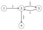
Figure 1.21:A network with a source and a sink
The middle left panel of Figure 1.20 shows the hub-based eigenvector centrality ranking for the international credit network shown in Figure 1.14. Countries that are rated highly according to this rank tend to be important players in terms of supply of credit. Japan takes the highest rank according to this measure, although countries with large financial sectors such as Great Britain and France are not far behind. (The color scheme in Figure 1.14 is also matched to hub-based eigenvector centrality.)
The authority-based eigenvector centrality of is defined as the solving
The difference between (1.34) and (1.32) is just transposition of . (Transposes do not affect the spectral radius of a matrix.) Element-by-element, this is
We see will be high if many nodes with high authority rankings link to .
The middle right panel of Figure 1.20 shows the authority-based eigenvector centrality ranking for the international credit network shown in Figure 1.14. Highly ranked countries are those that attract large inflows of credit, or credit inflows from other major players. The US clearly dominates the rankings as a target of interbank credit.
1.4.3.5Katz Centrality¶
Eigenvector centrality can be problematic. Although the definition in (1.32) makes sense when is strongly connected (so that, by the Perron–Frobenius theorem, ), strong connectedness fails in many real world networks. We will see examples of this in Section 2.1, for production networks defined by input-output matrices.
In addition, while strong connectedness yields strict positivity of the dominant eigenvector, many vertices can be assigned a zero ranking when it fails (see, e.g., Exercise 1.4.7). This zero ranking often runs counter to our intuition when we examine specific networks.
Considerations such as these encourage use of an alternative notion of centrality for networks called Katz centrality, originally due to Katz (1953), which is positive under weaker conditions and uniquely defined up to a tuning parameter. Fixing in , the hub-based Katz centrality of weighted digraph with adjacency matrix , at parameter , is defined as the vector that solves
The intuition is very similar to that provided for eigenvector centrality: high centrality is conferred on when it is linked to by vertices that themselves have high centrality. The difference between (1.36) and (1.32) is just in the additive constant .
The attenuation parameter is used to ensure that is finite and uniquely defined under the condition . It can be proved that, when the graph is strongly connected, hub-based (resp., authority-based) Katz centrality converges to the hub-based (resp., authority-based) eigenvector centrality as .[17] This is why, in the bottom two panels of Figure 1.20, the hub-based (resp., authority-based) Katz centrality ranking is seen to be close to its eigenvector-based counterpart.
When , we use as the default for Katz centrality computations.
Analogously, the authority-based Katz centrality of is defined as the that solves
1.4.4Scale-Free Networks¶
What kinds of properties do large, complex networks typically possess? One of the most striking facts about complex networks is that many exhibit the scale-free property, which means, loosely speaking, that the number of connections possessed by each vertex in the network follows a power law. The scale-free property is remarkable because it holds for a wide variety of networks, from social networks to citation, sales, financial and production networks, each of which is generated by different underlying mechanisms. Nonetheless, they share this specific statistical structure.
We begin this section by defining the degree distribution and then discuss its properties, including possible power law behavior.
1.4.4.1Empirical Degree Distributions¶
Let be a digraph. Assuming without loss of generality that for some , the in-degree distribution of is the sequence defined by
where is the in-degree of vertex . In other words, the in-degree distribution evaluated at is the fraction of nodes in the network that have in-degree . In Python, when is expressed as a Networkx DiGraph called G and import numpy as np has been executed, the in-degree distribution can be calculated via
def in_degree_dist(G):
n = G.number_of_nodes()
iG = np.array([G.in_degree(v) for v in G.nodes()])
phi = [np.mean(iG == k) for k in range(n+1)]
return phiThe out-degree distribution is defined analogously, replacing with in (1.40), and denoted by .
Recall that a digraph is called undirected if implies . If is undirected, then for all . In this case we usually write instead of or and refer simply to the degree-distribution of the digraph.
A scale-free network is a network whose degree distribution obeys a power law, in the sense that there exist positive constants and with
Here can refer to in-degree or the out-degree (or both), depending on our interest. In view of the discussion in Section 1.3.2.4, this can be identified with the idea that the degree distribution is Pareto-tailed with tail index .
Although we omit formal tests, the degree distribution for the commercial aircraft international trade network shown in Figure 1.2 is approximately scale-free. Figure 1.22 illustrates this by plotting the degree distribution alongside with and . (In this calculation of the degree distribution, performed by the Networkx function degree_histogram, directions are ignored and the network is treated as an undirected graph.)
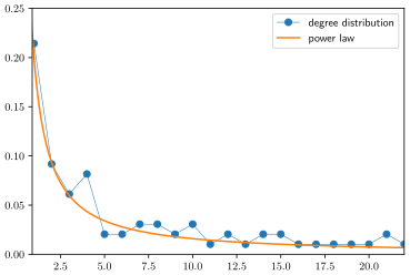
Figure 1.22:Degree distribution for international aircraft trade
Attention was drawn to the scale-free nature of many networks by Barabási & Albert (1999). They found, for example, that the in-degree and out-degree distributions for internet pages connected by hyperlinks both follow power laws. In subsequent years, many networks have been found to have the scale-free property, up to a first approximation, including networks of followers on Twitter Pearce, 2017Punel & Ermagun, 2018, other social networks Rybski et al., 2009 and academic collaboration networks (e.g., papers plus citations).
Within economics and finance, Carvalho (2014) shows that the weighted out-degree distribution for US input-output data (discussed further in Chapter 2) obeys a power law, as does the Katz centrality measure. Carvalho et al. (2021) document power law tails for the in-degree (suppliers) and out-degree (customers) distributions in a Japanese network of interacting firms. Scale-free degree distributions have also been observed in a number of financial and inter-bank credit networks Kim et al., 2007Ou et al., 2007De Masi et al., 2011.
In many cases, the scale-free property of a given network has significant implications for economic outcomes and welfare. For example, a power law in input-output networks often typically indicates dominance by a small number of very large sectors or firms. This in turn affects both the dynamism of industry and the likelihood of aggregate instability caused by firm-level shocks. We explore some of these issues in Chapter 2.
1.4.4.2Random Graphs¶
One way to explore the implications of different dynamics for the degree distribution of graphs is to specify a law for generating graphs randomly and then examine the degree distribution that results. This methodology leads to insights on the kinds of mechanisms that can generate scale-free networks.
We begin with one of the most popular and elementary ways of randomly generating an undirected graph, originally examined by Erdös & Rényi (1960). The process to generate a graph is
fix an integer and a ,
view as a collection of vertices,
let , and
for each with , add the undirected edge to the set of edges with probability .
In the last step additions are independent—each time, we flip an unbiased IID coin with head probability and add the edge if the coin comes up heads.
The Python code below provides a function that can be called to randomly generate an undirected graph using this procedure. It applies the combinations function from the itertools library, which, for the call combinations(A, k), returns a list of all subsets of of size . For example,
import itertools
letters = 'a', 'b', 'c'
list(itertools.combinations(letters, 2)) returns [(’a’, ’b’), (’a’, ’c’), (’b’, ’c’)].
We use combinations to produce the set of all possible edges and then add them to the graph with probability :
def erdos_renyi_graph(n=100, p=0.5, seed=1234):
"Returns an Erdos-Renyi random graph."
np.random.seed(seed)
edges = itertools.combinations(range(n), 2)
G = nx.Graph()
for e in edges:
if np.random.rand() < p:
G.add_edge(*e)
return G(The code presented here is a simplified version of functionality provided by the library Networkx. It is written for clarity rather than efficiency. More efficient versions can be found both in Networkx and in Julia’s Graphs.jl library.)
The left hand side of Figure 1.23 shows one instance of a graph that was generated by the erdos_renyi_graph function, with and . Lighter colors on a node indicate higher degree (more connections). The right hand side shows the degree distribution, which exhibits a bell-shaped curve typical for Erdos–Renyi random graphs. In fact one can show (see, e.g., Bollobás (1999) or Durrett (2007)) that the degree distribution is binomial, with
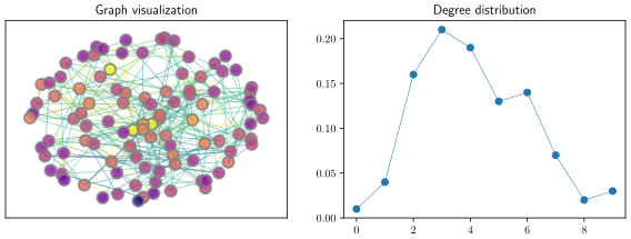
Figure 1.23:An instance of an Erdos–Renyi random graph
1.4.4.3Preferential Attachment¶
Clearly Erdos–Renyi random graphs fail to replicate the heavy right hand tail of the degree distribution observed in many networks. In response to this, Barabási & Albert (1999) proposed a mechanism for randomly generating graphs that feature the scale-free property.
The stochastic mechanism they proposed is called preferential attachment. In essence, each time a new vertex is added to an undirected graph, it is attached by edges to of the existing vertices, where the probability of vertex being selected is proportional to the degree of . Barabási & Albert (1999) showed that the resulting degree distribution exhibits a Pareto tail in the limit, as the number of vertices converges to . A careful proof can be found in Chapter 4 of Durrett (2007).
Although we omit details of the proof, we can see the power law emerge in simulations. For example, Figure 1.24 shows a random graph with 100 nodes generated by Networkx’s barabasi_albert_graph function. The number of attachments is set to 5. The simulated degree distribution on the right hand side of Figure 1.24 already exhibits a long right tail.
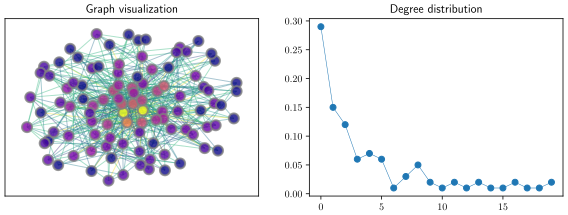
Figure 1.24:An instance of a preferential attachment random graph
The preferential attachment model is popular not just because it replicates the scale-free property of many real-world networks, but also because its mechanism is simple and plausible. For example, in citation networks, we can imagine that a well-cited paper is more likely to attract additional citations than a poorly-cited paper. Similar intuition can be applied to an individual on a social network, where the number of links is measured in terms of the number of followers.
1.5Chapter Notes¶
The Perron–Frobenius theorem is due to Oskar Perron (1880–1975) and Ferdinand Georg Frobenius (1849–1917). The main results were proved by 1912. As early as 1915, Dénes König (1884–1944) saw the connection between the Perron–Frobenius theorem and graph theory, and provided an alternative proof using bipartite graphs. Some of the history is discussed in Schrijver (2005).
We have already mentioned the textbooks on economic and social networks by Jackson (2010), Easley & Kleinberg (2010), Borgatti et al. (2018), and Goyal (2023), as well as the handbook by Bramoullé et al. (2016). Jackson (2014) gives a survey of the literature. Within the realm of network science, the high level texts by Newman (2018), Menczer et al. (2020) and Coscia (2021) are excellent.
One good text on graphs and graph-theoretic algorithms is Kepner & Gilbert (2011). Ballester et al. (2006) provide an interpretation of Katz centrality (which they call Bonacich centrality) in terms of Nash equilibria of quadratic games. Sharkey (2017) presents a new interpretation of Katz centrality using control theory. Polovnikov et al. (2022) use Katz centrality to uncover hidden ultimate owners in firm ownership data. Du et al. (2015) show how PageRank can be obtained as a competitive equilibrium of an economic problem. Calvó-Armengol et al. (2009) develop a model in which the outcomes for agents embedded in a network are proportional to the Katz centrality. Elliott & Golub (2019) show that, in a setting where agents can create nonrival, heterogeneous public goods, an important set of efficient solutions are characterized by contributions being proportional to agents’ eigenvector centralities in the network.
Kumamoto & Kamihigashi (2018) provide a detailed survey of power laws in economics and social sciences, including a discussion of the preferential attachment model of Barabási & Albert (1999). Newman (2005) is also highly readable. The textbook of Durrett (2007) is rigorous, carefully written and contains interesting motivational background, as well as an extensive citation list for studies of scale-free networks.
It should be clear from the symbol in (1.41) that the definition of scale-free networks is not entirely rigorous. Moreover, when connecting the definition to observed networks, we cannot obtain complete clarity by taking a limit, as we did when we defined power laws in Section 1.3.2, since the number of vertices is always finite. This imprecision in the definition has led to heated debate (see, e.g., Holme (2019)). Given the preponderance of positive empirical studies, we take the view that, up to a reasonable degree of approximation, the scale-free property is remarkably widespread.
In Section 1.4.2.3 we briefly mentioned network games, social networks and key players. These topics deserve more attention than we are able to provide. An excellent overview is given in Zenou (2016). Amarasinghe et al. (2020) apply these ideas to problems in economic development. Valuable related papers include Allouch (2015), Belhaj et al. (2016), Demange (2017), Belhaj & Deroı̈an (2019), Galeotti et al. (2020).
Another topic we reluctantly omit in order to keep the textbook short is endogenous network formation in economic environments. Influential papers in this field include Bala & Goyal (2000), Watts (2001), Graham (2017), Galeotti & Goyal (2010), Hojman & Szeidl (2008), and Jackson & Wolinsky (1996).
Finally, Candogan et al. (2012) study the profit maximization problem for a monopolist who sells items to participants in a social network. The main idea is that, in certain settings, the monopolist will find it profitable to offer discounts to key players in the network. Atalay et al. (2011) argue that in-degrees observed in US buyer-supplier networks have lighter tails than a power law, and supply a model that better fits their data.
This figure was constructed by QuantEcon research fellow Matthew McKay, using International Trade Data (SITC, Rev 2) collected by The Growth Lab at Harvard University.
This figure was also constructed by Matthew McKay, using data 2019 International Trade Data SITC Revision 2, code 7924. The data pertains to trade in commercial aircraft weighted at least 15,000kg. It was sourced from CID Dataverse.
See Section 6.1.3 for a discussion of big O notation.
See, for example, Jänich (1994), Chapter 6.
The only concern with this shift process is that can be ill-conditioned, implying that the inverse is numerically unstable.
See also Glynn & Desai (2018), which provides a new proof of the main results, based on probabilistic arguments, including extensions to infinite state spaces.
The probability is the same no matter whether inequalities are weak or strict.
Stationary distributions of stochastic matrices were intensively studied by many mathematicians well over a century before Larry Page and Sergey Brin patented the PageRank algorithm, so it seems unfair to allow them to appropriate the name.
Terminology on heavy tails varies across the literature but our choice is increasingly standard. See, for example, Foss et al. (2011) or Nair et al. (2021).
Obviously the correct value of depends on , so we can write for some suitable function . The correct function for this normalization is called the Riemann zeta function.
Graph theory is often regarded as originating from work by the brilliant Swiss mathematician Leonhard Euler (1707–1783), including his famous paper on the “Seven Bridges of Königsberg.”
Note that, in some applied fields, the adjacency matrix is transposed: if there is an edge from to , rather than from to . We will avoid this odd and confusing definition (which contradicts both standard graph theory and standard notational conventions in the study of Markov chains).
Data for the figure was obtained from the BIS consolidated banking statistics, for Q4 of 2022. Our calculations used the immediate counterparty basis for financial claims of domestic and foreign banks, which calculates the sum of cross-border claims and local claims of foreign affiliates in both foreign and local currency. The foreign claim of a node to itself is set to zero.
In fact arrows representing foreign claims less than US$10 million are cut from Figure 1.14, so the network is even denser than it appears.
Centrality measures are sometimes called “influence measures,” particularly in connection with social networks.
While the dominant eigenvector is only defined up to a positive scaling constant, this is no reason for concern, since positive scaling has no impact on the ranking. In most cases, users of this centrality ranking choose the dominant eigenvector satisfying .
See, for example, Benzi & Klymko (2015).
- Carvalho, V. M., & Grassi, B. (2019). Large firm dynamics and the business cycle. American Economic Review, 109(4), 1375–1425.
- Cohen, M. X. (2021). Linear Algebra: Theory, Intuition, Code. sincXpress.
- Jänich, K. (1994). Linear algebra. Undergraduate Texts in Mathematics. Springer-Verlag, New York, 7, 8.
- Cheney, W. (2013). Analysis for applied mathematics (Vol. 208). Springer Science & Business Media.
- Meyer, C. D. (2000). Matrix analysis and applied linear algebra (Vol. 71). Siam.
- Seneta, E. (2006). Non-negative matrices and Markov chains. Springer Science & Business Media.
- Meyer-Nieberg, P. (2012). Banach lattices. Springer Science & Business Media.
- Çınlar, E. (2011). Probability and stochastics (Vol. 261). Springer Science & Business Media.
- Häggström, O. (2002). Finite Markov chains and algorithmic applications. Cambridge University Press.
- Norris, J. R. (1998). Markov chains. Cambridge university press.
- Acemoglu, D., Ozdaglar, A., & Tahbaz-Salehi, A. (2016). Networks, Shocks, and Systemic Risk. In The Oxford Handbook of the Economics of Networks. Oxford.
- Zenou, Y. (2016). Key players. Oxford Handbook on the Economics of Networks, 244–274.
- Benzi, M., & Klymko, C. (2015). On the limiting behavior of parameter-dependent network centrality measures. SIAM Journal on Matrix Analysis and Applications, 36(2), 686–706.
- Katz, L. (1953). A new status index derived from sociometric analysis. Psychometrika, 18(1), 39–43.
- Barabási, A.-L., & Albert, R. (1999). Emergence of scaling in random networks. Science, 286(5439), 509–512.