120. 长寿、异质性个体、世代交叠模型#
GPU
本讲座是在配有GPU的机器上构建的——不过没有GPU也可以运行。
Google Colab 提供带GPU的免费套餐,使用方法如下:
点击右上角的”播放”图标
选择 Colab
将运行时环境设置为包含GPU
除了Anaconda中已有的库之外,本讲座还需要以下库
!pip install jax
120.1. 概述#
本讲座描述了一个具有以下特征的世代交叠模型:
不完全市场的竞争均衡决定价格和数量
如 [Auerbach and Kotlikoff, 1987] 所述,个体存活多个时期
如 [Aiyagari, 1994] 所述,个体受到无法完全投保的特殊劳动生产率冲击
如 [Auerbach and Kotlikoff, 1987] 第2章和 Transitions in an Overlapping Generations Model 所述,政府财政政策工具包括税率、债务和转移支付
在其他均衡要素中,竞争均衡决定了异质性个体消费、劳动收入和储蓄的横截面密度序列
我们使用该模型研究:
财政政策如何影响不同世代
市场不完全性如何促进预防性储蓄
生命周期储蓄和缓冲储蓄动机如何相互作用
财政政策如何在世代间和世代内重新分配资源
作为本讲座的先决条件,我们推荐两个 quantecon 讲座:
以及可选阅读材料 艾亚加里模型
像往常一样,让我们先导入一些 Python 模块
from collections import namedtuple
import numpy as np
import matplotlib.pyplot as plt
import matplotlib as mpl
FONTPATH = "fonts/SourceHanSerifSC-SemiBold.otf"
mpl.font_manager.fontManager.addfont(FONTPATH)
plt.rcParams['font.family'] = ['Source Han Serif SC']
import jax.numpy as jnp
import jax.scipy as jsp
import jax
120.2. 经济环境#
我们首先介绍我们所处的经济环境。
120.2.1. 人口统计和时间#
我们在离散时间中工作,用 \(t = 0, 1, 2, ...\) 表示。
每个个体存活 \(J = 50\) 个时期,不存在死亡风险。
我们用 \(j = 0, 1, ..., 49\) 表示年龄,人口规模固定在 \(1/J\)。
120.2.2. 个体状态变量#
在时间 \(t\) 时,年龄为 \(j\) 的个体 \(i\) 由两个状态变量表征:资产持有量 \(a_{i,j,t}\) 和特质劳动生产率 \(\gamma_{i,j,t}\)。
特质劳动生产率过程遵循一个两状态马尔可夫链,取值为 \(\gamma_l\) 和 \(\gamma_h\),转移矩阵为 \(\Pi\)。
新生个体在这些生产率状态上的初始分布为 \(\pi = [0.5, 0.5]\)。
120.2.3. 劳动供给#
生产率为 \(\gamma_{i,j,t}\) 的个体提供 \(l(j)\gamma_{i,j,t}\) 单位的有效劳动。
\(l(j)\) 是一个确定性的年龄特定劳动效率单位曲线。
个体的有效劳动供给取决于生命周期效率曲线和特质随机过程。
120.2.4. 初始条件#
新生个体的初始资产为零 \(a_{i,0,t} = 0\)。
初始特质生产率从分布 \(\pi\) 中抽取。
个体不留遗产,终期价值函数为 \(V_J(a) = 0\)。
120.3. 生产#
代表性企业采用规模报酬不变的柯布-道格拉斯生产函数:
其中:
\(K_t\) 是总资本
\(L_t\) 是总劳动效率单位
\(Z_t\) 是全要素生产率
\(\alpha\) 是资本份额
120.4. 政府#
政府实行包括债务、税收、转移支付和政府支出的财政政策。
政府发行一期债务 \(D_t\) 来为其运营提供资金,并通过对劳动和资本收入征收统一税率 \(\tau_t\) 来收取收入。
政府还实施针对不同年龄组的定额税收或转移支付 \(\delta_{j,t}\),可以在不同年龄组之间重新分配资源。
此外,政府还进行公共物品和服务的政府采购 \(G_t\)。
政府在时间 \(t\) 的预算约束是
其中总税收 \(T_t\) 满足
120.5. 要素市场活动#
在每个时间 \(t \geq 0\),个体供应劳动和资本。
120.5.1. 特定年龄的劳动供给#
年龄为 \(j \in \{0,1,...,J-1\}\) 的个体根据以下因素供应劳动:
其确定性的年龄效率曲线 \(l(j)\)
其当前特质生产率冲击 \(\gamma_{i,j,t}\)
每个个体供应 \(l(j)\gamma_{i,j,t}\) 个有效劳动单位,并按每个有效单位获得竞争性工资 \(w_t\),同时需缴纳统一税率 \(\tau_t\) 的劳动收入税。
120.5.2. 资产市场参与#
总结资产市场活动,所有年龄为 \(j \in \{0,1,...,J-1\}\) 的个体都可以:
持有资产 \(a_{i,j,t}\)(受借贷约束)
在储蓄上获得无风险的单期回报率 \(r_t\)
按统一税率 \(\tau_t\) 缴纳资本所得税
获得或支付与年龄相关的转移支付 \(\delta_{j,t}\)
120.5.3. 主要特征#
生命周期模式影响不同年龄的经济行为:
劳动生产率根据年龄曲线 \(l(j)\) 系统性变化,而资产持有量通常遵循工作年龄段积累、退休年龄段消耗的生命周期模式。
特定年龄的财政转移支付 \(\delta_{j,t}\) 在代际间重新分配资源。
同期群组内部异质性导致同龄人之间的差异:
同龄人因特异性生产率冲击的不同历史、当前生产率 \(\gamma_{i,j,t}\),以及由此产生的劳动收入和金融财富的差异,而在资产持有量 \(a_{i,j,t}\) 上存在差异。
跨期群组互动通过市场聚合决定均衡结果:
所有群组共同参与要素市场,所有群组的资产供给决定总资本,所有群组的有效劳动供给决定总劳动。
均衡价格反映生命周期和再分配的双重力量。
120.6. 代表性企业的问题#
代表性企业选择资本和有效劳动以最大化利润
一阶必要条件意味着
和
120.7. 家庭问题#
家庭的价值函数满足贝尔曼方程
其中最大化受约束于
以及终端条件 \(V_{J,t}(a, \gamma) = 0\)
120.8. 人口动态#
资产持有量和特质劳动生产率的联合概率密度函数\(\mu_{j,t}(a,\gamma)\)按如下方式演化:
对于新生人口\((j=0)\):
对于其他群组:
\[ \mu_{j+1,t+1}(a',\gamma') = \int {\bf 1}_{\sigma_{j,t}(a,\gamma)=a'}\Pi(\gamma,\gamma')\mu_{j,t}(a,\gamma)d(a,\gamma) \]
其中\(\sigma_{j,t}(a,\gamma)\)是最优储蓄策略函数。
120.9. 均衡#
均衡包括:
价值函数\(V_{j,t}\)
策略函数\(\sigma_{j,t}\)
联合概率分布\(\mu_{j,t}\)
价格\(r_t, w_t\)
政府政策\(\tau_t, D_t, \delta_{j,t}, G_t\)
满足以下条件:
在给定价格和政府政策的情况下,价值函数和策略函数解决家庭问题
在给定价格的情况下,代表性企业实现利润最大化
政府预算约束得到满足
市场出清:
资产市场:\(K_t = \sum_j \int a \mu_{j,t}(a,\gamma)d(a,\gamma) - D_t\)
劳动力市场:\(L_t = \sum_j \int l(j)\gamma \mu_{j,t}(a,\gamma)d(a,\gamma)\)
相对于Transitions in an Overlapping Generations Model中提出的模型,本模型增加了:
由生产率冲击导致的代内异质性
预防性储蓄动机
更多的再分配效应
更复杂的转型动态
120.10. 实现#
使用Discrete State Dynamic Programming中的工具,我们通过将值函数迭代与均衡价格确定相结合来求解我们的模型。
一个合理的方法是在寻找市场出清价格的外循环中嵌套一个离散动态规划求解器。
对于候选序列的利率\(r_t\)和工资\(w_t\),我们可以使用值函数迭代或策略迭代来求解个体家庭的动态规划问题,从而获得最优策略函数。
然后我们推导出每个年龄群体的资产持有量和特质劳动效率单位的相关平稳联合概率分布。
这将给我们提供总资本供给(来自家庭储蓄)和劳动力供给(来自年龄效率曲线和生产率冲击)。
然后我们可以将这些与企业的资本和劳动力需求进行比较,计算要素市场供给和需求之间的偏差,然后更新价格猜测,直到找到市场出清价格。
为了构建转型动态,我们可以通过使用_向后归纳法_计算价值函数和政策函数,以及使用_向前迭代法_计算主体在各状态之间的分布,来计算时变价格序列:
外循环(市场出清)
猜测初始价格(\(r_t, w_t\))
迭代直到资产和劳动力市场出清
使用企业的一阶必要条件来更新价格
内循环(个体动态规划)
对每个年龄群组:
离散化资产和生产率状态空间
使用价值函数迭代或政策迭代
求解最优储蓄政策
计算稳态分布
聚合
在每个群组内对个体状态求和
跨群组求和得到
总资本供给,和
总有效劳动力供给
考虑人口权重 \(1/J\)
转型动态
向后归纳:
从最终稳态开始
求解价值函数序列
向前迭代:
从初始分布开始
追踪群组分布随时间变化
每期市场出清:
求解价格序列
更新直到所有市场在所有期都出清
我们通过定义描述偏好、企业和政府预算约束的辅助函数来开始编码。
ϕ, k_bar = 0., 0.

@jax.jit
def V_bar(a):
    "根据资产持有量确定的终端价值函数。"

    return - ϕ * (a - k_bar) ** 2
ν = 0.5

@jax.jit
def u(c):
    "消费带来的效用。"

    return c ** (1 - ν) / (1 - ν)

l1, l2, l3 = 0.5, 0.05, -0.0008

@jax.jit
def l(j):
    "年龄相关的工资曲线。"

    return l1 + l2 * j + l3 * j ** 2
让我们定义一个包含控制生产技术参数的Firm命名元组。
Firm = namedtuple("Firm", ("α", "Z"))

def create_firm(α=0.3, Z=1):

    return Firm(α=α, Z=Z)
firm = create_firm()
以下辅助函数将从代表性企业的一阶必要条件中得出的要素投入(\(K, L\))和要素价格(\(w, r\))联系起来。
@jax.jit
def KL_to_r(K, L, firm):

    α, Z = firm

    return Z * α * (K / L) ** (α - 1)

@jax.jit
def KL_to_w(K, L, firm):

    α, Z = firm

    return Z * (1 - α) * (K / L) ** α
我们使用函数find_τ来寻找能够平衡政府预算约束的统一税率,这个税率取决于其他政策变量,包括债务水平、政府支出和转移支付。
@jax.jit
def find_τ(policy, price, aggs):

    D, D_next, G, δ = policy
    r, w = price
    K, L = aggs

    num = r * D + G - D_next + D - δ.sum(axis=-1)
    denom = w * L + r * (D + K)

    return num / denom
我们使用命名元组Household来存储表征家庭问题的参数。
Household = namedtuple("Household", ("j_grid", "a_grid", "γ_grid",
                                     "Π", "β", "init_μ", "VJ"))

def create_household(
        a_min=0., a_max=10, a_size=200,
        Π=[[0.9, 0.1], [0.1, 0.9]],
        γ_grid=[0.5, 1.5],
        β=0.96, J=50
    ):

    j_grid = jnp.arange(J)

    a_grid = jnp.linspace(a_min, a_max, a_size)

    γ_grid, Π = map(jnp.array, (γ_grid, Π))
    γ_size = len(γ_grid)

    # 新生人口的分布
    init_μ = jnp.zeros((a_size * γ_size))

    # 新生者的初始资产为零
    # 且γ的概率相等
    init_μ = init_μ.at[:γ_size].set(1 / γ_size)

    # 终端值V_bar(a)
    VJ = jnp.empty(a_size * γ_size)
    for a_i in range(a_size):
        a = a_grid[a_i]
        VJ = VJ.at[a_i*γ_size:(a_i+1)*γ_size].set(V_bar(a))

    return Household(j_grid=j_grid, a_grid=a_grid, γ_grid=γ_grid,
                     Π=Π, β=β, init_μ=init_μ, VJ=VJ)
hh = create_household()
我们应用离散状态动态规划工具。
初始步骤包括为我们的离散化贝尔曼方程准备奖励矩阵 \(R\) 和转移矩阵 \(Q\)。
@jax.jit
def populate_Q(household):

    j_grid, a_grid, γ_grid, Π, β, init_μ, VJ = household

    num_state = a_grid.size * γ_grid.size
    num_action = a_grid.size

    Q = jsp.linalg.block_diag(*[Π]*a_grid.size)
    Q = Q.reshape((num_state, num_action, γ_grid.size))
    Q = jnp.tile(Q, a_grid.size).T

    return Q

@jax.jit
def populate_R(j, r, w, τ, δ, household):

    j_grid, a_grid, γ_grid, Π, β, init_μ, VJ = household

    num_state = a_grid.size * γ_grid.size
    num_action = a_grid.size

    a = jnp.reshape(a_grid, (a_grid.size, 1, 1))
    γ = jnp.reshape(γ_grid, (1, γ_grid.size, 1))
    ap = jnp.reshape(a_grid, (1, 1, a_grid.size))
    c = (1 + r*(1-τ)) * a + (1-τ) * w * l(j) * γ - δ[j] - ap

    return jnp.reshape(jnp.where(c > 0, u(c), -jnp.inf),
                      (num_state, num_action))
120.11. 计算稳态#
我们首先计算一个稳态。
给定价格和税收的猜测值,我们可以使用反向归纳法来求解所有年龄段的价值函数以及最优消费和储蓄策略。
函数backwards_opt通过反向应用离散化的贝尔曼算子来求解最优值。
我们使用jax.lax.scan来高效地进行顺序和递归计算。
@jax.jit
def backwards_opt(prices, taxes, household, Q):

    r, w = prices
    τ, δ = taxes

    j_grid, a_grid, γ_grid, Π, β, init_μ, VJ = household
    J = j_grid.size

    num_state = a_grid.size * γ_grid.size
    num_action = a_grid.size

    def bellman_operator_j(V_next, j):
        "在给定Vj+1的情况下,求解年龄j时的家庭优化问题"

        Rj = populate_R(j, r, w, τ, δ, household)
        vals = Rj + β * Q.dot(V_next)
        σ_j = jnp.argmax(vals, axis=1)
        V_j = vals[jnp.arange(num_state), σ_j]

        return V_j, (V_j, σ_j)

    js = jnp.arange(J-1, -1, -1)
    init_V = VJ

    # 从年龄J迭代到1
    _, outputs = jax.lax.scan(bellman_operator_j, init_V, js)
    V, σ = outputs
    V = V[::-1]
    σ = σ[::-1]

    return V, σ
r, w = 0.05, 1
τ, δ = 0.15, np.zeros(hh.j_grid.size)

Q = populate_Q(hh)
V, σ = backwards_opt([r, w], [τ, δ], hh, Q)
让我们用 block_until_ready() 来计时,以确保所有 JAX 运算都已完成
%time backwards_opt([r, w], [τ, δ], hh, Q)[0].block_until_ready();
CPU times: user 1.44 s, sys: 2.02 ms, total: 1.44 s
Wall time: 373 ms
从每个群组的最优消费和储蓄选择出发,我们可以计算出稳态下资产水平和特质生产率水平的联合概率分布。
@jax.jit
def popu_dist(σ, household, Q):

    j_grid, a_grid, γ_grid, Π, β, init_μ, VJ = household

    J = hh.j_grid.size
    num_state = hh.a_grid.size * hh.γ_grid.size

    def update_popu_j(μ_j, j):
        "更新从年龄j到j+1的人口分布"

        Qσ = Q[jnp.arange(num_state), σ[j]]
        μ_next = μ_j @ Qσ

        return μ_next, μ_next

    js = jnp.arange(J-1)

    # 从年龄1迭代到J
    _, μ = jax.lax.scan(update_popu_j, init_μ, js)
    μ = jnp.concatenate([init_μ[jnp.newaxis], μ], axis=0)

    return μ
μ = popu_dist(σ, hh, Q)
让我们计时计算过程
%time popu_dist(σ, hh, Q)[0].block_until_ready();
CPU times: user 32.7 ms, sys: 0 ns, total: 32.7 ms
Wall time: 29.2 ms
下面我们绘制每个年龄组的储蓄边缘分布。
for j in [0, 5, 20, 45, 49]:
    plt.plot(hh.a_grid, jnp.sum(μ[j].reshape((hh.a_grid.size, hh.γ_grid.size)), axis=1), label=f'j={j}')

plt.legend()
plt.xlabel('a')

plt.title(r'marginal distribution over a, $\sum_\gamma \mu_j(a, \gamma)$')
plt.xlim([0, 8])
plt.ylim([0, 0.1])

plt.show()
findfont: Failed to find font weight normal, now using 600.
findfont: Failed to find font weight normal, now using 600.
findfont: Failed to find font weight normal, now using 600.
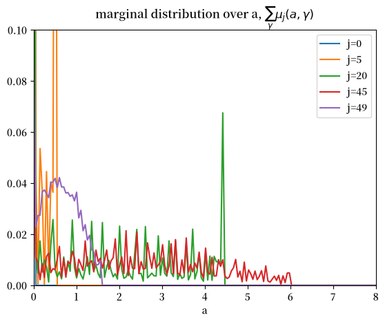
这些边缘分布确认新进入经济体的个体没有任何资产持有。
蓝色的 \(j=0\) 分布仅在 \(a=0\) 处有质量。
随着个体年龄增长,他们最初会逐渐积累资产。
橙色的 \(j=5\) 分布在正但较低的资产水平上有正质量
绿色的 \(j=20\) 分布在更广范围的资产水平上有正质量
红色的 \(j=45\) 分布范围更宽
在较晚年龄,他们会逐渐减少其资产持有。
紫色的 \(j=49\) 分布说明了这一点
在生命末期,他们将耗尽所有资产。
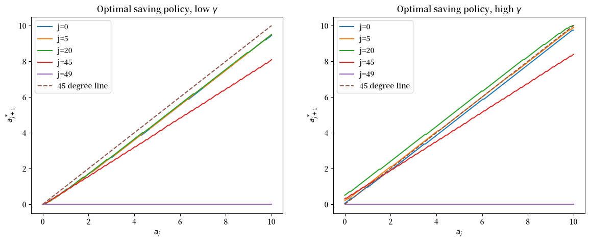
让我们现在看看产生前述不同年龄资产边缘分布的年龄特定最优储蓄政策。
我们将用以下Python代码绘制一些储蓄函数。
σ_reshaped = σ.reshape(hh.j_grid.size, hh.a_grid.size, hh.γ_grid.size)
j_labels = [f'j={j}' for j in [0, 5, 20, 45, 49]]

fig, axs = plt.subplots(1, 2, figsize=(14, 5))

axs[0].plot(hh.a_grid, hh.a_grid[σ_reshaped[[0, 5, 20, 45, 49], :, 0].T])
axs[0].plot(hh.a_grid, hh.a_grid, '--')
axs[0].set_xlabel("$a_{j}$")
axs[0].set_ylabel("$a^*_{j+1}$")
axs[0].legend(j_labels+['45 degree line'])
axs[0].set_title(r"Optimal saving policy, low $\gamma$")

axs[1].plot(hh.a_grid, hh.a_grid[σ_reshaped[[0, 5, 20, 45, 49], :, 1].T])
axs[1].plot(hh.a_grid, hh.a_grid, '--')
axs[1].set_xlabel("$a_{j}$")
axs[1].set_ylabel("$a^*_{j+1}$")
axs[1].legend(j_labels+['45 degree line'])
axs[1].set_title(r"Optimal saving policy, high $\gamma$")

plt.show()
findfont: Failed to find font weight normal, now using 600.
从隐含的平稳人口分布中,我们可以计算总劳动供给 \(L\) 和私人储蓄 \(A\)。
@jax.jit
def compute_aggregates(μ, household):

    j_grid, a_grid, γ_grid, Π, β, init_μ, VJ = household

    J, a_size, γ_size = j_grid.size, a_grid.size, γ_grid.size

    μ = μ.reshape((J, hh.a_grid.size, hh.γ_grid.size))

    # 计算私人储蓄
    a = a_grid.reshape((1, a_size, 1))
    A = (a * μ).sum() / J

    γ = γ_grid.reshape((1, 1, γ_size))
    lj = l(j_grid).reshape((J, 1, 1))
    L = (lj * γ * μ).sum() / J

    return A, L
A, L = compute_aggregates(μ, hh)
A, L
(Array(1.8592227, dtype=float32), Array(1.0781993, dtype=float32))
该经济体中的资本存量等于\(A-D\)。
D = 0
K = A - D
企业的最优条件意味着利率 \(r\) 和工资率 \(w\)。
KL_to_r(K, L, firm), KL_to_w(K, L, firm)
(Array(0.20487012, dtype=float32), Array(0.82430464, dtype=float32))
隐含价格\((r,w)\)与我们的猜测不同,所以我们必须更新猜测并迭代直到找到一个不动点。
这是我们的外层循环。
@jax.jit
def find_ss(household, firm, pol_target, Q, tol=1e-6, verbose=False):

    j_grid, a_grid, γ_grid, Π, β, init_μ, VJ = household
    J = j_grid.size
    num_state = a_grid.size * γ_grid.size

    D, G, δ = pol_target

    # 价格的初始猜测
    r, w = 0.05, 1.

    # τ的初始猜测
    τ = 0.15

    def cond_fn(state):
        "收敛标准。"

        V, σ, μ, K, L, r, w, τ, D, G, δ, r_old, w_old = state

        error = (r - r_old) ** 2 + (w - w_old) ** 2

        return error > tol

    def body_fn(state):
        "迭代的主体部分。"

        V, σ, μ, K, L, r, w, τ, D, G, δ, r_old, w_old = state
        r_old, w_old, τ_old = r, w, τ

        # 家庭最优决策和价值
        V, σ = backwards_opt([r, w], [τ, δ], hh, Q)

        # 计算稳态分布
        μ = popu_dist(σ, hh, Q)

        # 计算总量
        A, L = compute_aggregates(μ, hh)
        K = A - D

        # 更新价格
        r, w = KL_to_r(K, L, firm), KL_to_w(K, L, firm)

        # 寻找τ
        D_next = D
        τ = find_τ([D, D_next, G, δ],
                   [r, w],
                   [K, L])

        r = (r + r_old) / 2
        w = (w + w_old) / 2

        return V, σ, μ, K, L, r, w, τ, D, G, δ, r_old, w_old

    # 初始状态
    V = jnp.empty((J, num_state), dtype=float)
    σ = jnp.empty((J, num_state), dtype=int)
    μ = jnp.empty((J, num_state), dtype=float)

    K, L = 1., 1.
    initial_state = (V, σ, μ, K, L, r, w, τ, D, G, δ, r-1, w-1)
    V, σ, μ, K, L, r, w, τ, D, G, δ, _, _ = jax.lax.while_loop(
                                    cond_fn, body_fn, initial_state)

    return V, σ, μ, K, L, r, w, τ, D, G, δ
ss1 = find_ss(hh, firm, [0, 0.1, np.zeros(hh.j_grid.size)], Q, verbose=True)
让我们计时计算过程
%time find_ss(hh, firm, [0, 0.1, np.zeros(hh.j_grid.size)], Q)[0].block_until_ready();
CPU times: user 12.5 s, sys: 36.1 ms, total: 12.5 s
Wall time: 3.24 s
hh_out_ss1 = ss1[:3]
quant_ss1 = ss1[3:5]
price_ss1 = ss1[5:7]
policy_ss1 = ss1[7:11]
# V, σ, μ
V_ss1, σ_ss1, μ_ss1 = hh_out_ss1
# K, L
K_ss1, L_ss1 = quant_ss1

K_ss1, L_ss1
(Array(6.619442, dtype=float32), Array(1.0781994, dtype=float32))
# 利率,工资
r_ss1, w_ss1 = price_ss1

r_ss1, w_ss1
(Array(0.08426618, dtype=float32), Array(1.2060944, dtype=float32))
# τ, D, G, δ
τ_ss1, D_ss1, G_ss1, δ_ss1 = policy_ss1

τ_ss1, D_ss1, G_ss1, δ_ss1
(Array(0.05381015, dtype=float32),
 Array(0, dtype=int32, weak_type=True),
 Array(0.1, dtype=float32, weak_type=True),
 Array([0., 0., 0., 0., 0., 0., 0., 0., 0., 0., 0., 0., 0., 0., 0., 0., 0.,
        0., 0., 0., 0., 0., 0., 0., 0., 0., 0., 0., 0., 0., 0., 0., 0., 0.,
        0., 0., 0., 0., 0., 0., 0., 0., 0., 0., 0., 0., 0., 0., 0., 0.],      dtype=float32))
120.12. 转换动态#
我们使用path_iteration函数计算转换动态。
在外循环中,我们对价格和税收的猜测值进行迭代。
在内循环中,我们计算每个年龄组\(j\)在每个时间\(t\)的最优消费和储蓄选择,然后找出资产和生产力联合分布的隐含演变。
然后,我们根据经济中的总劳动供给和资本存量更新价格和税收的猜测值。
我们使用solve_backwards来求解给定价格和税收序列下的最优储蓄选择,并使用simulate_forward来计算联合分布的演变。
我们需要两个稳态作为输入:初始稳态为simulate_forward提供初始条件,最终稳态为solve_backwards提供延续值。
@jax.jit
def bellman_operator(prices, taxes, V_next, household, Q):

    r, w = prices
    τ, δ = taxes

    j_grid, a_grid, γ_grid, Π, β, init_μ, VJ = household
    J = j_grid.size

    num_state = a_grid.size * γ_grid.size
    num_action = a_grid.size

    def bellman_operator_j(j):
        Rj = populate_R(j, r, w, τ, δ, household)
        vals = Rj + β * Q.dot(V_next[j+1])
        σ_j = jnp.argmax(vals, axis=1)
        V_j = vals[jnp.arange(num_state), σ_j]

        return V_j, σ_j

    V, σ = jax.vmap(bellman_operator_j, (0,))(jnp.arange(J-1))

    # 最后的生命阶段
    j = J-1
    Rj = populate_R(j, r, w, τ, δ, household)
    vals = Rj + β * Q.dot(VJ)
    σ = jnp.concatenate([σ, jnp.argmax(vals, axis=1)[jnp.newaxis]])
    V = jnp.concatenate([V, vals[jnp.arange(num_state), σ[j]][jnp.newaxis]])

    return V, σ
@jax.jit
def solve_backwards(V_ss2, σ_ss2, household, firm, price_seq, pol_seq, Q):

    j_grid, a_grid, γ_grid, Π, β, init_μ, VJ = household
    J = j_grid.size
    num_state = a_grid.size * γ_grid.size

    τ_seq, D_seq, G_seq, δ_seq = pol_seq
    r_seq, w_seq = price_seq

    T = r_seq.size

    def solve_backwards_t(V_next, t):

        prices = (r_seq[t], w_seq[t])
        taxes = (τ_seq[t], δ_seq[t])
        V, σ = bellman_operator(prices, taxes, V_next, household, Q)

        return V, (V,σ)

    ts = jnp.arange(T-2, -1, -1)
    init_V = V_ss2

    _, outputs = jax.lax.scan(solve_backwards_t, init_V, ts)
    V_seq, σ_seq = outputs
    V_seq = V_seq[::-1]
    σ_seq = σ_seq[::-1]

    V_seq = jnp.concatenate([V_seq, V_ss2[jnp.newaxis]])
    σ_seq = jnp.concatenate([σ_seq, σ_ss2[jnp.newaxis]])

    return V_seq, σ_seq
@jax.jit
def population_evolution(σt, μt, household, Q):

    j_grid, a_grid, γ_grid, Π, β, init_μ, VJ = household

    J = hh.j_grid.size
    num_state = hh.a_grid.size * hh.γ_grid.size

    def population_evolution_j(j):

        Qσ = Q[jnp.arange(num_state), σt[j]]
        μ_next = μt[j] @ Qσ

        return μ_next

    μ_next = jax.vmap(population_evolution_j, (0,))(jnp.arange(J-1))
    μ_next = jnp.concatenate([init_μ[jnp.newaxis], μ_next])

    return μ_next
@jax.jit
def simulate_forwards(σ_seq, D_seq, μ_ss1, K_ss1, L_ss1, household, Q):

    j_grid, a_grid, γ_grid, Π, β, init_μ, VJ = household

    J, num_state = μ_ss1.shape

    T = σ_seq.shape[0]

    def simulate_forwards_t(μ, t):

        μ_next = population_evolution(σ_seq[t], μ, household, Q)

        A, L = compute_aggregates(μ_next, household)
        K = A - D_seq[t+1]

        return μ_next, (μ_next, K, L)

    ts = jnp.arange(T-1)
    init_μ = μ_ss1

    _, outputs = jax.lax.scan(simulate_forwards_t, init_μ, ts)
    μ_seq, K_seq, L_seq = outputs

    μ_seq = jnp.concatenate([μ_ss1[jnp.newaxis], μ_seq])
    K_seq = jnp.concatenate([K_ss1[jnp.newaxis], K_seq])
    L_seq = jnp.concatenate([L_ss1[jnp.newaxis], L_seq])

    return μ_seq, K_seq, L_seq
以下算法描述了路径迭代程序:
算法 120.1 (AK-Aiyagari过渡路径算法)
输入 给定初始稳态\(ss_1\),最终稳态\(ss_2\),时间范围\(T\),和政策序列\((D, G, \delta)\)
输出 计算价值函数\(V\)、政策函数\(\sigma\)、分布\(\mu\)和价格\((r, w, \tau)\)的均衡过渡路径
从稳态初始化:
\((V_1, \sigma_1, \mu_1) \leftarrow ss_1\) (初始稳态)
\((V_2, \sigma_2, \mu_2) \leftarrow ss_2\) (最终稳态)
\((r, w, \tau) \leftarrow initialize\_prices(T)\) (线性插值)
\(error \leftarrow \infty\), \(i \leftarrow 0\)
当 \(error > \varepsilon\) 或 \(i \leq max\_iter\) 时:
\(i \leftarrow i + 1\)
\((r_{\text{old}}, w_{\text{old}}, \tau_{\text{old}}) \leftarrow (r, w, \tau)\)
向后归纳: 对于 \(t \in [T, 1]\):
对于 \(j \in [0, J-1]\) (年龄组):
\(V[t,j] \leftarrow \max_{a'} \{u(c) + \beta\mathbb{E}[V[t+1,j+1]]\}\)
\(\sigma[t,j] \leftarrow \arg\max_{a'} \{u(c) + \beta\mathbb{E}[V[t+1,j+1]]\}\)
向前模拟: 对于 \(t \in [1, T]\):
\(\mu[t] \leftarrow \Gamma(\sigma[t], \mu[t-1])\) (分布演化)
\(K[t] \leftarrow \int a \, d\mu[t] - D[t]\) (总资本)
\(L[t] \leftarrow \int l(j)\gamma \, d\mu[t]\) (总劳动)
\(r[t] \leftarrow \alpha Z(K[t]/L[t])^{\alpha-1}\) (利率)
\(w[t] \leftarrow (1-\alpha)Z(K[t]/L[t])^{\alpha}\) (工资率)
\(\tau[t] \leftarrow solve\_budget(r[t],w[t],K[t],L[t],D[t],G[t])\)
计算收敛指标:
\(error \leftarrow \|r - r_{\text{old}}\| + \|w - w_{\text{old}}\| + \|\tau - \tau_{\text{old}}\|\)
使用阻尼更新价格:
\(r \leftarrow \lambda r + (1-\lambda)r_{\text{old}}\)
\(w \leftarrow \lambda w + (1-\lambda)w_{\text{old}}\)
\(\tau \leftarrow \lambda \tau + (1-\lambda)\tau_{\text{old}}\)
返回 \((V, \sigma, \mu, r, w, \tau)\)
def path_iteration(ss1, ss2, pol_target, household, firm, Q, tol=1e-4, verbose=False):

    # 起点:初始稳态
    V_ss1, σ_ss1, μ_ss1 = ss1[:3]
    K_ss1, L_ss1 = ss1[3:5]
    r_ss1, w_ss1 = ss1[5:7]
    τ_ss1, D_ss1, G_ss1, δ_ss1 = ss1[7:11]

    # 终点:收敛的新稳态
    V_ss2, σ_ss2, μ_ss2 = ss2[:3]
    K_ss2, L_ss2 = ss2[3:5]
    r_ss2, w_ss2 = ss2[5:7]
    τ_ss2, D_ss2, G_ss2, δ_ss2 = ss2[7:11]

    # 给定的政策:D, G, δ
    D_seq, G_seq, δ_seq = pol_target
    T = G_seq.shape[0]

    # 价格的初始猜测
    r_seq = jnp.linspace(0, 1, T) * (r_ss2 - r_ss1) + r_ss1
    w_seq = jnp.linspace(0, 1, T) * (w_ss2 - w_ss1) + w_ss1

    # 政策的初始猜测
    τ_seq = jnp.linspace(0, 1, T) * (τ_ss2 - τ_ss1) + τ_ss1

    error = 1
    num_iter = 0

    if verbose:
        fig, axs = plt.subplots(1, 3, figsize=(14, 3))
        axs[0].plot(jnp.arange(T), r_seq)
        axs[1].plot(jnp.arange(T), w_seq)
        axs[2].plot(jnp.arange(T), τ_seq, label=f'iter {num_iter}')

    while error > tol:
        # 重复直到找到不动点

        r_old, w_old, τ_old = r_seq, w_seq, τ_seq

        pol_seq = (τ_seq, D_seq, G_seq, δ_seq)
        price_seq = (r_seq, w_seq)

        # 向后求解最优政策
        V_seq, σ_seq = solve_backwards(
            V_ss2, σ_ss2, hh, firm, price_seq, pol_seq, Q)

        # 向前计算人口演变
        μ_seq, K_seq, L_seq = simulate_forwards(
            σ_seq, D_seq, μ_ss1, K_ss1, L_ss1, household, Q)

        # 根据总资本和劳动供给更新价格
        r_seq = KL_to_r(K_seq, L_seq, firm)
        w_seq = KL_to_w(K_seq, L_seq, firm)

        # 找到平衡政府预算约束的税率
        τ_seq = find_τ([D_seq[:-1], D_seq[1:], G_seq, δ_seq],
                       [r_seq, w_seq],
                       [K_seq, L_seq])

        # 新旧猜测之间的距离
        error = jnp.sum((r_old - r_seq) ** 2) + \
                jnp.sum((w_old - w_seq) ** 2) + \
                jnp.sum((τ_old - τ_seq) ** 2)

        num_iter += 1
        if verbose:
            print(f"迭代 {num_iter:3d}: error = {error:.6e}")
            axs[0].plot(jnp.arange(T), r_seq)
            axs[1].plot(jnp.arange(T), w_seq)
            axs[2].plot(jnp.arange(T), τ_seq, label=f'iter {num_iter}')

        r_seq = (r_seq + r_old) / 2
        w_seq = (w_seq + w_old) / 2
        τ_seq = (τ_seq + τ_old) / 2

    if verbose:
        axs[0].set_xlabel('t')
        axs[1].set_xlabel('t')
        axs[2].set_xlabel('t')

        axs[0].set_title('r')
        axs[1].set_title('w')
        axs[2].set_title('τ')

        axs[2].legend(loc='center left', bbox_to_anchor=(1, 0.5))

    return V_seq, σ_seq, μ_seq, K_seq, L_seq, r_seq, w_seq, \
            τ_seq, D_seq, G_seq, δ_seq
现在我们可以计算由财政政策改革引发的均衡转换。
120.13. 实验1:即时减税#
假设政府降低税率,并通过发行债务立即平衡其预算。
在\(t=0\)时,政府出人意料地宣布立即减税。
从\(t=0\)到\(19\),政府发行债务,因此债务\(D_{t+1}\)在20个周期内呈线性增长。
政府为其新债务水平设定目标\(D_{20} =D_0 + 1 = \bar{D} + 1\)。
政府支出\(\bar{G}\)和转移支付\(\bar{\delta}_j\)保持不变。
政府调整\(\tau_t\)以在转换过程中平衡预算。
我们要计算均衡转换路径。
我们的第一步是准备适当的政策变量数组D_seq、G_seq、δ_seq
我们将计算一个能平衡政府预算的τ_seq。
T = 150

D_seq = jnp.ones(T+1) * D_ss1
D_seq = D_seq.at[:21].set(D_ss1 + jnp.linspace(0, 1, 21))
D_seq = D_seq.at[21:].set(D_seq[20])

G_seq = jnp.ones(T) * G_ss1

δ_seq = jnp.repeat(δ_ss1, T).reshape((T, δ_ss1.size))
为了迭代路径,我们首先需要找到其目标点,也就是在新财政政策下的新稳态。
ss2 = find_ss(hh, firm, [D_seq[-1], G_seq[-1], δ_seq[-1]], Q)
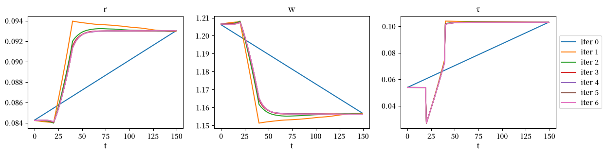
我们可以使用path_iteration来寻找均衡转移动态。
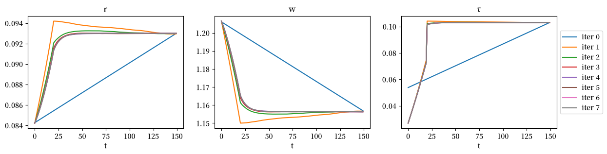
通过设置关键参数verbose=True,可以让函数path_iteration显示收敛信息。
paths = path_iteration(ss1, ss2, [D_seq, G_seq, δ_seq], hh, firm, Q, verbose=True)
迭代   1: error = 2.101515e-01
迭代   2: error = 3.756374e-02
迭代   3: error = 7.719551e-03
迭代   4: error = 1.821420e-03
迭代   5: error = 4.767649e-04
迭代   6: error = 1.218046e-04
迭代   7: error = 2.983156e-05
在成功计算了转型动态后,让我们来研究它们。
V_seq, σ_seq, μ_seq = paths[:3]
K_seq, L_seq = paths[3:5]
r_seq, w_seq = paths[5:7]
τ_seq, D_seq, G_seq, δ_seq = paths[7:11]
ap = hh.a_grid[σ_seq[0]]
j = jnp.reshape(hh.j_grid, (hh.j_grid.size, 1, 1))
lj = l(j)
a = jnp.reshape(hh.a_grid, (1, hh.a_grid.size, 1))
γ = jnp.reshape(hh.γ_grid, (1, 1, hh.γ_grid.size))
t = 0

ap = hh.a_grid[σ_seq[t]]
δ = δ_seq[t].reshape((hh.j_grid.size, 1, 1))

inc = (1 + r_seq[t]*(1-τ_seq[t])) * a \
        + (1-τ_seq[t]) * w_seq[t] * lj * γ - δ
inc = inc.reshape((hh.j_grid.size, hh.a_grid.size * hh.γ_grid.size))

c = inc - ap

c_mean0 = (c * μ_seq[t]).sum(axis=1)
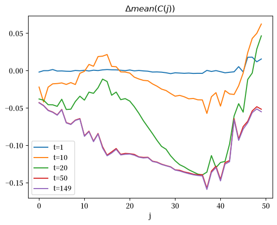
我们关注政策变化如何影响不同年龄群体和不同时期的消费。
我们可以研究特定年龄的平均消费水平。
for t in [1, 10, 20, 50, 149]:

    ap = hh.a_grid[σ_seq[t]]
    δ = δ_seq[t].reshape((hh.j_grid.size, 1, 1))

    inc = (1 + r_seq[t]*(1-τ_seq[t])) * a + (1-τ_seq[t]) * w_seq[t] * lj * γ - δ
    inc = inc.reshape((hh.j_grid.size, hh.a_grid.size * hh.γ_grid.size))

    c = inc - ap

    c_mean = (c * μ_seq[t]).sum(axis=1)

    plt.plot(range(hh.j_grid.size), c_mean-c_mean0, label=f't={t}')

plt.legend()
plt.xlabel(r'j')
plt.title(r'$\Delta mean(C(j))$')
plt.show()
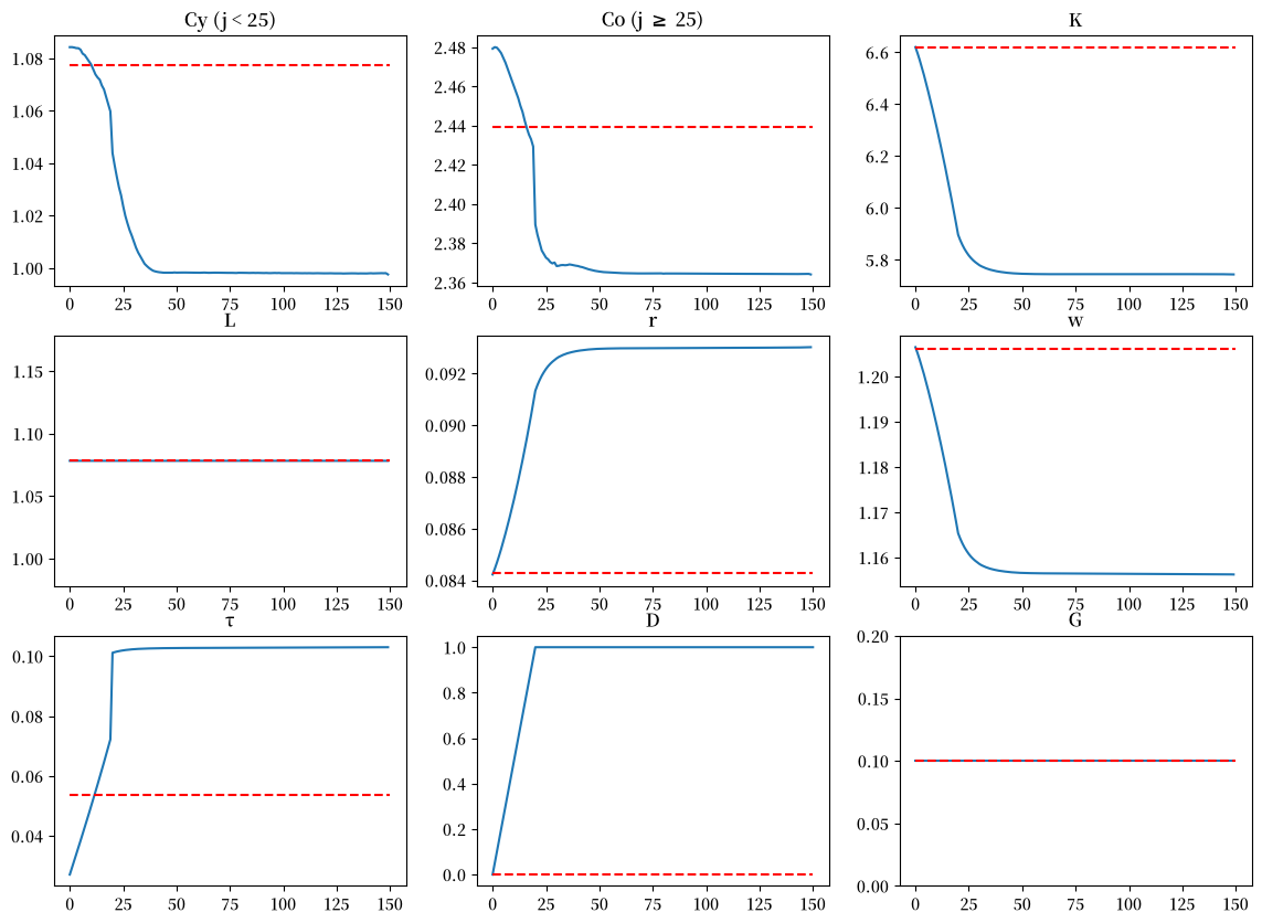
为了总结这个转变过程,我们可以像在代际交叠模型中的转型中那样绘制路径。
但与那个两期生命的世代交叠模型设置不同,我们现在不再有具有代表性的老年和年轻主体。
现在我们在每个时间点都有50个不同年龄的群组
为了继续,我们构建两个规模相等的年龄组 – 年轻组和老年组。
在25岁时,一个人从年轻组转变为老年组
ap = hh.a_grid[σ_ss1]
J = hh.j_grid.size
δ = δ_ss1.reshape((hh.j_grid.size, 1, 1))

inc = (1 + r_ss1*(1-τ_ss1)) * a + (1-τ_ss1) * w_ss1 * lj * γ - δ
inc = inc.reshape((hh.j_grid.size, hh.a_grid.size * hh.γ_grid.size))

c = inc - ap

Cy_ss1 = (c[:J//2] * μ_ss1[:J//2]).sum() / (J // 2)
Co_ss1 = (c[J//2:] * μ_ss1[J//2:]).sum() / (J // 2)
T = σ_seq.shape[0]
J = σ_seq.shape[1]

Cy_seq = np.empty(T)
Co_seq = np.empty(T)

for t in range(T):
    ap = hh.a_grid[σ_seq[t]]
    δ = δ_seq[t].reshape((hh.j_grid.size, 1, 1))

    inc = (1 + r_seq[t]*(1-τ_seq[t])) * a + (1-τ_seq[t]) * w_seq[t] * lj * γ - δ
    inc = inc.reshape((hh.j_grid.size, hh.a_grid.size * hh.γ_grid.size))

    c = inc - ap

    Cy_seq[t] = (c[:J//2] * μ_seq[t, :J//2]).sum() / (J // 2)
    Co_seq[t] = (c[J//2:] * μ_seq[t, J//2:]).sum() / (J // 2)
fig, axs = plt.subplots(3, 3, figsize=(14, 10))

# Cy (j=0-24)
axs[0, 0].plot(Cy_seq)
axs[0, 0].hlines(Cy_ss1, 0, T, color='r', linestyle='--')
axs[0, 0].set_title('Cy (j < 25)')

# Cy (j=25-49)
axs[0, 1].plot(Co_seq)
axs[0, 1].hlines(Co_ss1, 0, T, color='r', linestyle='--')
axs[0, 1].set_title(r'Co (j $\geq$ 25)')

names = ['K', 'L', 'r', 'w', 'τ', 'D', 'G']
for i in range(len(names)):
    i_var = i + 3
    i_axes = i + 2

    row_i = i_axes // 3
    col_i = i_axes % 3

    axs[row_i, col_i].plot(paths[i_var])
    axs[row_i, col_i].hlines(ss1[i_var], 0, T, color='r', linestyle='--')
    axs[row_i, col_i].set_title(names[i])

# y轴范围
axs[1, 0].set_ylim([ss1[4]-0.1, ss1[4]+0.1])
axs[2, 2].set_ylim([ss1[9]-0.1, ss1[9]+0.1])

plt.show()
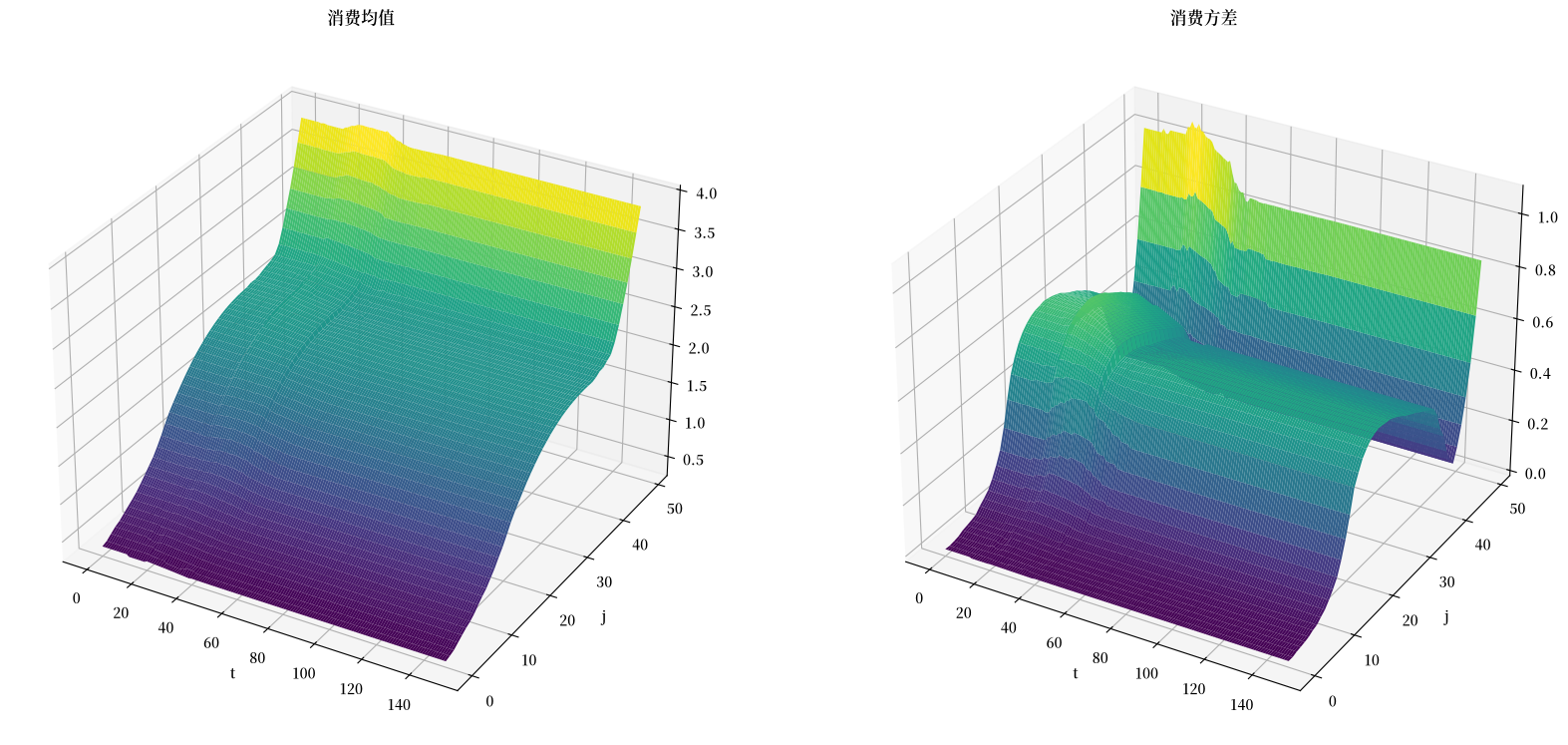
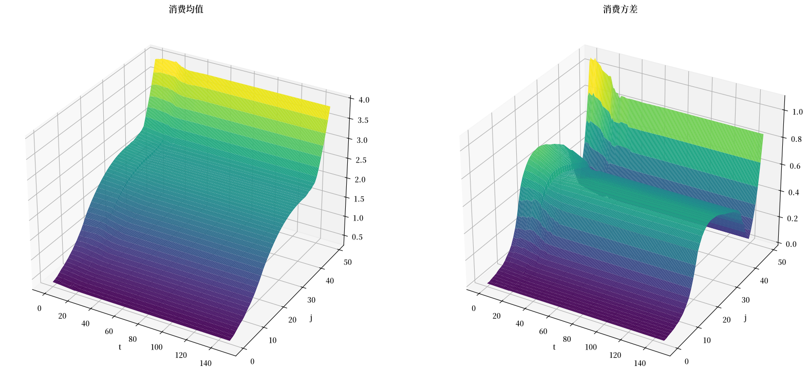
现在让我们计算每个时间点\(t\)下基于年龄的条件消费均值和方差。
Cmean_seq = np.empty((T, J))
Cvar_seq = np.empty((T, J))

for t in range(T):
    ap = hh.a_grid[σ_seq[t]]
    δ = δ_seq[t].reshape((hh.j_grid.size, 1, 1))

    inc = (1 + r_seq[t]*(1-τ_seq[t])) * a + (1-τ_seq[t]) * w_seq[t] * lj * γ - δ
    inc = inc.reshape((hh.j_grid.size, hh.a_grid.size * hh.γ_grid.size))

    c = inc - ap

    Cmean_seq[t] = (c * μ_seq[t]).sum(axis=1)
    Cvar_seq[t] = ((c - Cmean_seq[t].reshape((J, 1))) ** 2 * μ_seq[t]).sum(axis=1)
J_seq, T_range = np.meshgrid(np.arange(J), np.arange(T))

fig = plt.figure(figsize=[20, 20])

# 绘制消费均值随年龄和时间的变化
ax1 = fig.add_subplot(121, projection='3d')
ax1.plot_surface(T_range, J_seq, Cmean_seq, rstride=1, cstride=1,
                cmap='viridis', edgecolor='none')
ax1.set_title(r"消费均值")
ax1.set_xlabel(r"t")
ax1.set_ylabel(r"j")

# 绘制消费方差随年龄和时间的变化
ax2 = fig.add_subplot(122, projection='3d')
ax2.plot_surface(T_range, J_seq, Cvar_seq, rstride=1, cstride=1,
                cmap='viridis', edgecolor='none')
ax2.set_title(r"消费方差")
ax2.set_xlabel(r"t")
ax2.set_ylabel(r"j")

plt.show()
120.14. 实验2:预先宣布的减税#
现在政府在时间\(0\)宣布永久性减税,但在20个周期后才实施。
我们将使用相同的关键工具path_iteration。
我们必须适当地指定D_seq。
T = 150

D_t = 20
D_seq = jnp.ones(T+1) * D_ss1
D_seq = D_seq.at[D_t:D_t+21].set(D_ss1 + jnp.linspace(0, 1, 21))
D_seq = D_seq.at[D_t+21:].set(D_seq[D_t+20])

G_seq = jnp.ones(T) * G_ss1

δ_seq = jnp.repeat(δ_ss1, T).reshape((T, δ_ss1.size))
ss2 = find_ss(hh, firm, [D_seq[-1], G_seq[-1], δ_seq[-1]], Q)
paths = path_iteration(ss1, ss2, [D_seq, G_seq, δ_seq],
                    hh, firm, Q, verbose=True)
迭代   1: error = 1.313959e-01
迭代   2: error = 2.366369e-02
迭代   3: error = 4.936778e-03
迭代   4: error = 1.197292e-03
迭代   5: error = 3.145675e-04
迭代   6: error = 7.859751e-05
V_seq, σ_seq, μ_seq = paths[:3]
K_seq, L_seq = paths[3:5]
r_seq, w_seq = paths[5:7]
τ_seq, D_seq, G_seq, δ_seq = paths[7:11]
T = σ_seq.shape[0]
J = σ_seq.shape[1]

Cy_seq = np.empty(T)
Co_seq = np.empty(T)

for t in range(T):
    ap = hh.a_grid[σ_seq[t]]
    δ = δ_seq[t].reshape((hh.j_grid.size, 1, 1))

    inc = (1 + r_seq[t]*(1-τ_seq[t])) * a + (1-τ_seq[t]) * w_seq[t] * lj * γ - δ
    inc = inc.reshape((hh.j_grid.size, hh.a_grid.size * hh.γ_grid.size))

    c = inc - ap

    Cy_seq[t] = (c[:J//2] * μ_seq[t, :J//2]).sum() / (J // 2)
    Co_seq[t] = (c[J//2:] * μ_seq[t, J//2:]).sum() / (J // 2)
下面我们绘制经济的转换路径。
fig, axs = plt.subplots(3, 3, figsize=(14, 10))

# Cy (j=0-24)
axs[0, 0].plot(Cy_seq)
axs[0, 0].hlines(Cy_ss1, 0, T, color='r', linestyle='--')
axs[0, 0].set_title('Cy (j < 25)')

# Cy (j=25-49)
axs[0, 1].plot(Co_seq)
axs[0, 1].hlines(Co_ss1, 0, T, color='r', linestyle='--')
axs[0, 1].set_title(r'Co (j $\geq$ 25)')

names = ['K', 'L', 'r', 'w', 'τ', 'D', 'G']
for i in range(len(names)):
    i_var = i + 3
    i_axes = i + 2

    row_i = i_axes // 3
    col_i = i_axes % 3

    axs[row_i, col_i].plot(paths[i_var])
    axs[row_i, col_i].hlines(ss1[i_var], 0, T, color='r', linestyle='--')
    axs[row_i, col_i].set_title(names[i])

# ylims
axs[1, 0].set_ylim([ss1[4]-0.1, ss1[4]+0.1])
axs[2, 2].set_ylim([ss1[9]-0.1, ss1[9]+0.1])

plt.show()
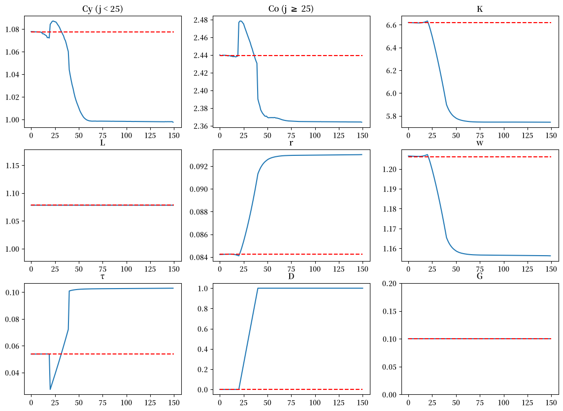
注意价格和数量是如何立即对预期的税率上调作出反应的。
让我们仔细观察资本存量是如何反应的。
# K
i_var = 3

plt.plot(paths[i_var][:25])
plt.hlines(ss1[i_var], 0, 25, color='r', linestyle='--')
plt.vlines(20, 6, 7, color='k', linestyle='--', linewidth=0.5)
plt.text(17, 6.56, r'tax cut')
plt.ylim([6.52, 6.65])
plt.title("K")
plt.xlabel("t")
plt.show()
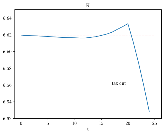
在t=20实施减税政策后,由于挤出效应,总资本将会减少。
个人在t=20之前几个时期就已预见到利率将会上升,因此开始增加储蓄。
由于储蓄的增加导致资本增加,随之而来的是利率的暂时下降。
对于生活在更早时期的个体来说,这种较低的利率使他们减少储蓄。
我们还可以沿着转换路径绘制不同群体消费的均值和方差的演变。
Cmean_seq = np.empty((T, J))
Cvar_seq = np.empty((T, J))

for t in range(T):
    ap = hh.a_grid[σ_seq[t]]
    δ = δ_seq[t].reshape((hh.j_grid.size, 1, 1))

    inc = (1 + r_seq[t]*(1-τ_seq[t])) * a + (1-τ_seq[t]) * w_seq[t] * lj * γ - δ
    inc = inc.reshape((hh.j_grid.size, hh.a_grid.size * hh.γ_grid.size))

    c = inc - ap

    Cmean_seq[t] = (c * μ_seq[t]).sum(axis=1)
    Cvar_seq[t] = (
        (c - Cmean_seq[t].reshape((J, 1))) ** 2 * μ_seq[t]).sum(axis=1)
J_seq, T_range = np.meshgrid(np.arange(J), np.arange(T))

fig = plt.figure(figsize=[20, 20])

# 绘制消费均值随年龄和时间的变化
ax1 = fig.add_subplot(121, projection='3d')
ax1.plot_surface(T_range, J_seq, Cmean_seq, rstride=1, cstride=1,
                cmap='viridis', edgecolor='none')
ax1.set_title(r"消费均值")
ax1.set_xlabel(r"t")
ax1.set_ylabel(r"j")

# 绘制消费方差随年龄和时间的变化
ax2 = fig.add_subplot(122, projection='3d')
ax2.plot_surface(T_range, J_seq, Cvar_seq, rstride=1, cstride=1,
                cmap='viridis', edgecolor='none')
ax2.set_title(r"消费方差")
ax2.set_xlabel(r"t")
ax2.set_ylabel(r"j")

plt.show()