72. 收入波动问题 II:乐观策略迭代#
GPU
本讲座是在配有GPU的机器上构建的——不过没有GPU也可以运行。
Google Colab 提供带GPU的免费套餐,使用方法如下:
点击右上角的”播放”图标
选择 Colab
将运行时环境设置为包含GPU
72.1. 概述#
在 收入波动问题 I:离散化与 VFI 中,我们研究了收入波动问题,并使用值函数迭代(VFI)求解了它。
在本讲座中,我们将使用 乐观策略迭代(OPI)来求解同一个问题。这种方法非常通用,通常比 VFI 更快,而且只是略微复杂一些。
OPI 结合了值函数迭代和策略迭代两者的要素。
关于该算法的详细讨论可以在 DP1 中找到。
我们的目标是实现 OPI,并测试它对于收入波动问题是否能相较于标准 VFI 带来显著的速度提升。
除了 Anaconda 之外,本讲座还需要以下库:
!pip install quantecon jax
我们将使用以下导入:
import quantecon as qe
import jax
import jax.numpy as jnp
import matplotlib.pyplot as plt
import matplotlib as mpl
FONTPATH = "fonts/SourceHanSerifSC-SemiBold.otf"
mpl.font_manager.fontManager.addfont(FONTPATH)
plt.rcParams['font.family'] = ['Source Han Serif SC']
from typing import NamedTuple
from time import time
72.2. 模型与基本要素#
模型和参数与 收入波动问题 I:离散化与 VFI 中的相同。
为方便起见,我们在这里重复关键要素。
家庭的问题是最大化
约束条件为
其中 \(u(c) = c^{1-\gamma}/(1-\gamma)\)。
以下是模型结构:
class Model(NamedTuple):
    β: float              # 贴现因子
    R: float              # 总利率
    γ: float              # CRRA 参数
    a_grid: jnp.ndarray   # 资产网格
    y_grid: jnp.ndarray   # 收入网格
    Q: jnp.ndarray        # 收入的马尔可夫矩阵


def create_consumption_model(
        R=1.01,                    # 总利率
        β=0.98,                    # 贴现因子
        γ=2,                       # CRRA 参数
        a_min=0.01,                # 最小资产
        a_max=10.0,                # 最大资产
        a_size=150,                # 网格大小
        ρ=0.9, ν=0.1, y_size=100   # 收入参数
    ):
    """
    Creates an instance of the consumption-savings model.

    """
    a_grid = jnp.linspace(a_min, a_max, a_size)
    mc = qe.tauchen(n=y_size, rho=ρ, sigma=ν)
    y_grid, Q = jnp.exp(mc.state_values), jax.device_put(mc.P)
    return Model(β, R, γ, a_grid, y_grid, Q)
72.3. 算子与策略#
我们重复 收入波动问题 I:离散化与 VFI 中的一些函数。
以下是贝尔曼方程的右侧:
def B(v, model, i, j, ip):
    """
    The right-hand side of the Bellman equation before maximization, which takes
    the form

        B(a, y, a′) = u(Ra + y - a′) + β Σ_y′ v(a′, y′) Q(y, y′)

    The indices are (i, j, ip) -> (a, y, a′).
    """
    β, R, γ, a_grid, y_grid, Q = model
    a, y, ap  = a_grid[i], y_grid[j], a_grid[ip]
    c = R * a + y - ap
    EV = jnp.sum(v[ip, :] * Q[j, :])
    return jnp.where(c > 0, c**(1-γ)/(1-γ) + β * EV, -jnp.inf)
现在我们依次应用 vmap 以在所有索引上进行向量化:
B_1    = jax.vmap(B,   in_axes=(None, None, None, None, 0))
B_2    = jax.vmap(B_1, in_axes=(None, None, None, 0,    None))
B_vmap = jax.vmap(B_2, in_axes=(None, None, 0,    None, None))
以下是贝尔曼算子:
def T(v, model):
    "The Bellman operator."
    a_indices = jnp.arange(len(model.a_grid))
    y_indices = jnp.arange(len(model.y_grid))
    B_values = B_vmap(v, model, a_indices, y_indices, a_indices)
    return jnp.max(B_values, axis=-1)
以下是计算 \(v\)-贪婪策略的函数:
def get_greedy(v, model):
    "Computes a v-greedy policy, returned as a set of indices."
    a_indices = jnp.arange(len(model.a_grid))
    y_indices = jnp.arange(len(model.y_grid))
    B_values = B_vmap(v, model, a_indices, y_indices, a_indices)
    return jnp.argmax(B_values, axis=-1)
现在我们定义策略算子 \(T_\sigma\),它是固定策略 \(\sigma\) 时的贝尔曼算子。
对于给定的策略 \(\sigma\),策略算子定义为
def T_σ(v, σ, model, i, j):
    """
    The σ-policy operator for indices (i, j) -> (a, y).
    """
    β, R, γ, a_grid, y_grid, Q = model

    # 获取当前状态下的值
    a, y = a_grid[i], y_grid[j]
    # 获取策略选择
    ap = a_grid[σ[i, j]]

    # 计算当前奖励
    c = R * a + y - ap
    r = jnp.where(c > 0, c**(1-γ)/(1-γ), -jnp.inf)

    # 计算期望值
    EV = jnp.sum(v[σ[i, j], :] * Q[j, :])

    return r + β * EV
应用 vmap 进行向量化:
T_σ_1    = jax.vmap(T_σ,   in_axes=(None, None, None, None, 0))
T_σ_vmap = jax.vmap(T_σ_1, in_axes=(None, None, None, 0,    None))

def T_σ_vec(v, σ, model):
    """Vectorized version of T_σ."""
    a_size, y_size = len(model.a_grid), len(model.y_grid)
    a_indices = jnp.arange(a_size)
    y_indices = jnp.arange(y_size)
    return T_σ_vmap(v, σ, model, a_indices, y_indices)
现在我们需要一个函数将策略算子应用 m 次:
def iterate_policy_operator(σ, v, m, model):
    """
    Apply the policy operator T_σ exactly m times to v.
    """
    def update(i, v):
        return T_σ_vec(v, σ, model)

    v = jax.lax.fori_loop(0, m, update, v)
    return v
72.4. 值函数迭代#
作为比较,以下是来自 收入波动问题 I:离散化与 VFI 的 VFI:
@jax.jit
def value_function_iteration(model, tol=1e-5, max_iter=10_000):
    """
    Implements VFI using successive approximation.
    """
    def body_fun(k_v_err):
        k, v, error = k_v_err
        v_new = T(v, model)
        error = jnp.max(jnp.abs(v_new - v))
        return k + 1, v_new, error

    def cond_fun(k_v_err):
        k, v, error = k_v_err
        return jnp.logical_and(error > tol, k < max_iter)

    v_init = jnp.zeros((len(model.a_grid), len(model.y_grid)))
    k, v_star, error = jax.lax.while_loop(cond_fun, body_fun,
                                          (1, v_init, tol + 1))
    return v_star, get_greedy(v_star, model)
72.5. 乐观策略迭代#
现在我们实现 OPI。
该算法在以下两步之间交替进行
执行 \(m\) 次策略算子迭代以更新值函数
基于更新后的值函数计算新的贪婪策略
@jax.jit
def optimistic_policy_iteration(model, m=10, tol=1e-5, max_iter=10_000):
    """
    Implements optimistic policy iteration with step size m.

    Parameters:
    -----------
    model : Model
        The consumption-savings model
    m : int
        Number of policy operator iterations per step
    tol : float
        Tolerance for convergence
    max_iter : int
        Maximum number of iterations
    """
    v_init = jnp.zeros((len(model.a_grid), len(model.y_grid)))

    def condition_function(inputs):
        i, v, error = inputs
        return jnp.logical_and(error > tol, i < max_iter)

    def update(inputs):
        i, v, error = inputs
        last_v = v
        σ = get_greedy(v, model)
        v = iterate_policy_operator(σ, v, m, model)
        error = jnp.max(jnp.abs(v - last_v))
        i += 1
        return i, v, error

    num_iter, v, error = jax.lax.while_loop(condition_function,
                                            update,
                                            (0, v_init, tol + 1))

    return v, get_greedy(v, model)
72.6. 计时比较#
让我们创建一个模型并比较 VFI 和 OPI 的性能。
model = create_consumption_model()
首先,让我们对 VFI 计时:
print("Starting VFI.")
start = time()
v_star_vfi, σ_star_vfi = value_function_iteration(model)
v_star_vfi.block_until_ready()
vfi_time_with_compile = time() - start
print(f"VFI completed in {vfi_time_with_compile:.2f} seconds.")
Starting VFI.
VFI completed in 0.50 seconds.
再次运行以消除编译时间:
start = time()
v_star_vfi, σ_star_vfi = value_function_iteration(model)
v_star_vfi.block_until_ready()
vfi_time = time() - start
print(f"VFI completed in {vfi_time:.2f} seconds.")
VFI completed in 0.35 seconds.
现在让我们用不同的 m 值对 OPI 计时:
print("Starting OPI with m=50.")
start = time()
v_star_opi, σ_star_opi = optimistic_policy_iteration(model, m=50)
v_star_opi.block_until_ready()
opi_time_with_compile = time() - start
print(f"OPI completed in {opi_time_with_compile:.2f} seconds.")
Starting OPI with m=50.
OPI completed in 0.50 seconds.
再次运行:
start = time()
v_star_opi, σ_star_opi = optimistic_policy_iteration(model, m=50)
v_star_opi.block_until_ready()
opi_time = time() - start
print(f"OPI completed in {opi_time:.2f} seconds.")
OPI completed in 0.30 seconds.
检查我们是否得到相同的结果:
print(f"Values match: {jnp.allclose(v_star_vfi, v_star_opi)}")
Values match: True
值函数相匹配,确认了两种算法收敛到相同的解。
让我们直观地比较两种策略下的资产动态:
fig, axes = plt.subplots(1, 2, figsize=(12, 5))

# VFI 策略
for j, label in zip([0, -1], ['低收入', '高收入']):
    a_next_vfi = model.a_grid[σ_star_vfi[:, j]]
    axes[0].plot(model.a_grid, a_next_vfi, label=label)
axes[0].plot(model.a_grid, model.a_grid, 'k--', linewidth=0.5, alpha=0.5)
axes[0].set(xlabel='当前资产', ylabel='下一期资产', title='VFI')
axes[0].legend()

# OPI 策略
for j, label in zip([0, -1], ['低收入', '高收入']):
    a_next_opi = model.a_grid[σ_star_opi[:, j]]
    axes[1].plot(model.a_grid, a_next_opi, label=label)
axes[1].plot(model.a_grid, model.a_grid, 'k--', linewidth=0.5, alpha=0.5)
axes[1].set(xlabel='当前资产', ylabel='下一期资产', title='OPI')
axes[1].legend()

plt.tight_layout()
plt.show()
findfont: Failed to find font weight normal, now using 600.
findfont: Failed to find font weight normal, now using 600.
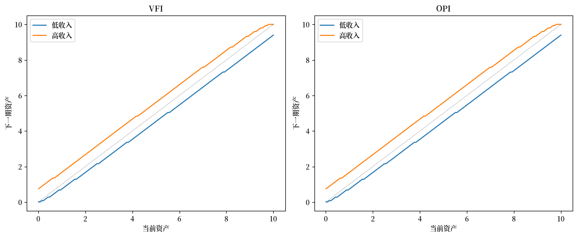
这两种策略在视觉上无法区分,确认了两种方法产生了相同的解。
以下是加速情况:
print(f"Speedup factor: {vfi_time / opi_time:.2f}")
Speedup factor: 1.17
让我们尝试不同的 m 值,看看它如何影响性能:
m_vals = [1, 5, 10, 25, 50, 100, 200, 400]
opi_times = []

for m in m_vals:
    start = time()
    v_star, σ_star = optimistic_policy_iteration(model, m=m)
    v_star.block_until_ready()
    elapsed = time() - start
    opi_times.append(elapsed)
    print(f"OPI with m={m:3d} completed in {elapsed:.2f} seconds.")
OPI with m=  1 completed in 2.39 seconds.
OPI with m=  5 completed in 0.72 seconds.
OPI with m= 10 completed in 0.49 seconds.
OPI with m= 25 completed in 0.37 seconds.
OPI with m= 50 completed in 0.30 seconds.
OPI with m=100 completed in 0.38 seconds.
OPI with m=200 completed in 0.64 seconds.
OPI with m=400 completed in 1.23 seconds.
绘制结果:
fig, ax = plt.subplots()
ax.plot(m_vals, opi_times, 'o-', label='OPI')
ax.axhline(vfi_time, linestyle='--', color='red', label='VFI')
ax.set_xlabel('m (每次迭代的策略步数)')
ax.set_ylabel('时间(秒)')
ax.legend()
ax.set_title('OPI 执行时间与步长 m 的关系')
plt.show()
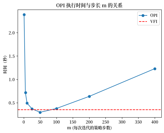
以下是结果的总结
OPI 在很大范围的 \(m\) 值上都优于 VFI。
对于非常大的 \(m\),OPI 的性能开始下降,因为我们在迭代策略算子上花费了过多时间。
72.7. 练习#
练习 72.1
OPI 所实现的速度提升对参数变化相当稳健。
请通过对收入过程的不同参数值(\(\rho\) 和 \(\nu\))进行实验来确认这一点。
测量它们如何影响 VFI 与 OPI 的相对性能。
尝试:
\(\rho \in \{0.8, 0.9, 0.95\}\)
\(\nu \in \{0.05, 0.1, 0.2\}\)
对于每种组合,计算加速因子(VFI 时间 / OPI 时间)并报告你的发现。
解答 练习 72.1
以下是一个解答:
ρ_vals = [0.8, 0.9, 0.95]
ν_vals = [0.05, 0.1, 0.2]

results = []

for ρ in ρ_vals:
    for ν in ν_vals:
        print(f"\nTesting ρ={ρ}, ν={ν}")

        # 创建模型
        model = create_consumption_model(ρ=ρ, ν=ν)

        # 对 VFI 计时
        start = time()
        v_vfi, σ_vfi = value_function_iteration(model)
        v_vfi.block_until_ready()
        vfi_t = time() - start

        # 对 OPI 计时
        start = time()
        v_opi, σ_opi = optimistic_policy_iteration(model, m=10)
        v_opi.block_until_ready()
        opi_t = time() - start

        speedup = vfi_t / opi_t
        results.append((ρ, ν, speedup))
        print(f"  VFI: {vfi_t:.2f}s, OPI: {opi_t:.2f}s, Speedup: {speedup:.2f}x")

# 打印总结
print("\nSummary of speedup factors:")
for ρ, ν, speedup in results:
    print(f"ρ={ρ}, ν={ν}: {speedup:.2f}x")
Testing ρ=0.8, ν=0.05
  VFI: 0.35s, OPI: 0.48s, Speedup: 0.73x

Testing ρ=0.8, ν=0.1
  VFI: 0.35s, OPI: 0.48s, Speedup: 0.72x

Testing ρ=0.8, ν=0.2
  VFI: 0.33s, OPI: 0.48s, Speedup: 0.69x

Testing ρ=0.9, ν=0.05
  VFI: 0.34s, OPI: 0.50s, Speedup: 0.68x

Testing ρ=0.9, ν=0.1
  VFI: 0.35s, OPI: 0.49s, Speedup: 0.72x

Testing ρ=0.9, ν=0.2
  VFI: 0.36s, OPI: 0.51s, Speedup: 0.70x

Testing ρ=0.95, ν=0.05
  VFI: 0.37s, OPI: 0.50s, Speedup: 0.73x

Testing ρ=0.95, ν=0.1
  VFI: 0.36s, OPI: 0.49s, Speedup: 0.73x

Testing ρ=0.95, ν=0.2
  VFI: 0.40s, OPI: 0.52s, Speedup: 0.78x

Summary of speedup factors:
ρ=0.8, ν=0.05: 0.73x
ρ=0.8, ν=0.1: 0.72x
ρ=0.8, ν=0.2: 0.69x
ρ=0.9, ν=0.05: 0.68x
ρ=0.9, ν=0.1: 0.72x
ρ=0.9, ν=0.2: 0.70x
ρ=0.95, ν=0.05: 0.73x
ρ=0.95, ν=0.1: 0.73x
ρ=0.95, ν=0.2: 0.78x