70. 最优储蓄 VI:使用 JAX 的 EGM#
GPU
本讲座是在配有GPU的机器上构建的——不过没有GPU也可以运行。
Google Colab 提供带GPU的免费套餐,使用方法如下:
点击右上角的”播放”图标
选择 Colab
将运行时环境设置为包含GPU
除了 Anaconda 中已有的内容外,本讲座还需要以下库:
!pip install quantecon jax
70.1. 概述#
在本讲座中,我们将使用 JAX 实现内生网格方法(EGM)。
本讲座建立在 最优储蓄 V:内生网格法 的基础上,该讲座使用 NumPy 介绍了 EGM。
通过转换为 JAX,我们可以利用快速线性代数、硬件加速器和 JIT 编译来提升性能。
我们还将使用 JAX 的 vmap 函数来完全向量化 Coleman-Reffett 算子。
让我们从一些标准导入开始:
import matplotlib.pyplot as plt
import jax
import jax.numpy as jnp
import quantecon as qe
from typing import NamedTuple
import matplotlib as mpl  # i18n
FONTPATH = "fonts/SourceHanSerifSC-SemiBold.otf"  # i18n
mpl.font_manager.fontManager.addfont(FONTPATH)  # i18n
mpl.rcParams['font.family'] = ['Source Han Serif SC']  # i18n
70.2. 实现#
关于储蓄问题和内生网格方法(EGM)的详细信息,请参见 最优储蓄 V:内生网格法。
这里我们专注于 EGM 的 JAX 实现。
我们使用与 最优储蓄 V:内生网格法 相同的设定:
\(u(c) = \ln c\),
生产是科布-道格拉斯型的,并且
冲击是对数正态的。
以下是用于比较的解析解。
def v_star(x, α, β, μ):
    """
    真实值函数
    """
    c1 = jnp.log(1 - α * β) / (1 - β)
    c2 = (μ + α * jnp.log(α * β)) / (1 - α)
    c3 = 1 / (1 - β)
    c4 = 1 / (1 - α * β)
    return c1 + c2 * (c3 - c4) + c4 * jnp.log(x)

def σ_star(x, α, β):
    """
    真实最优策略
    """
    return (1 - α * β) * x
Model 类仅存储数据(网格、冲击和参数)。
效用函数和生产函数将在全局定义,以便与 JAX 的 JIT 编译器协同工作。
class Model(NamedTuple):
    β: float              # 贴现因子
    μ: float              # 冲击位置参数
    s: float              # 冲击尺度参数
    s_grid: jnp.ndarray   # 外生储蓄网格
    shocks: jnp.ndarray   # 冲击抽样
    α: float              # 生产函数参数


def create_model(
        β: float = 0.96,
        μ: float = 0.0,
        s: float = 0.1,
        grid_max: float = 4.0,
        grid_size: int = 120,
        shock_size: int = 250,
        seed: int = 1234,
        α: float = 0.4
    ) -> Model:
    """
    创建最优储蓄模型的一个实例。
    """
    # 设置外生储蓄网格
    s_grid = jnp.linspace(1e-4, grid_max, grid_size)

    # 存储冲击(使用种子,以便结果可复现)
    key = jax.random.key(seed)
    shocks = jnp.exp(μ + s * jax.random.normal(key, shape=(shock_size,)))

    return Model(β, μ, s, s_grid, shocks, α)
我们在全局定义效用函数和生产函数。
# 定义效用函数和生产函数及其导数
u = lambda c: jnp.log(c)
u_prime = lambda c: 1 / c
u_prime_inv = lambda x: 1 / x
f = lambda k, α: k**α
f_prime = lambda k, α: α * k**(α - 1)
这是使用 EGM 的 Coleman-Reffett 算子。
这里的关键 JAX 特性是 vmap,它将计算向量化到各个网格点上。
def K(
        c_in: jnp.ndarray,  # 内生网格上的消费值
        x_in: jnp.ndarray,  # 当前内生网格
        model: Model        # 模型规格
    ):
    """
    使用 EGM 的 Coleman-Reffett 算子

    """
    β, μ, s, s_grid, shocks, α = model
    σ = lambda x_val: jnp.interp(x_val, x_in, c_in)

    # 定义在单个网格点上计算消费的函数
    def compute_c(s):
        # 近似边际效用 ∫ u'(σ(f(s, α)z)) f'(s, α) z ϕ(z)dz
        vals = u_prime(σ(f(s, α) * shocks)) * f_prime(s, α) * shocks
        mu = jnp.mean(vals)
        # 计算消费
        return u_prime_inv(β * mu)

    # 向量化并在所有外生网格点上计算
    compute_c_vectorized = jax.vmap(compute_c)
    c_out = compute_c_vectorized(s_grid)

    # 确定对应的内生网格
    x_out = s_grid + c_out  # x_i = s_i + c_i

    return c_out, x_out
现在我们创建一个模型实例。
model = create_model()
s_grid = model.s_grid
求解器使用 JAX 的 jax.lax.while_loop 进行迭代,并且经过 JIT 编译以提高速度。
@jax.jit
def solve_model_time_iter(
        model: Model,
        c_init: jnp.ndarray,
        x_init: jnp.ndarray,
        tol: float = 1e-5,
        max_iter: int = 1000
    ):
    """
    使用带 EGM 的时间迭代求解模型。
    """

    def condition(loop_state):
        i, c, x, error = loop_state
        return (error > tol) & (i < max_iter)

    def body(loop_state):
        i, c, x, error = loop_state
        c_new, x_new = K(c, x, model)
        error = jnp.max(jnp.abs(c_new - c))
        return i + 1, c_new, x_new, error

    # 初始化循环状态
    initial_state = (0, c_init, x_init, tol + 1)

    # 运行循环
    i, c, x, error = jax.lax.while_loop(condition, body, initial_state)

    return c, x
我们从一个初始猜测开始求解模型。
c_init = jnp.copy(s_grid)
x_init = s_grid + c_init
c, x = solve_model_time_iter(model, c_init, x_init)
让我们将得到的策略与解析解进行对比绘图。
fig, ax = plt.subplots()

ax.plot(x, c, lw=2,
        alpha=0.8, label='近似策略函数')

ax.plot(x, σ_star(x, model.α, model.β), 'k--',
        lw=2, alpha=0.8, label='真实策略函数')

ax.legend()
plt.show()
findfont: Failed to find font weight normal, now using 600.
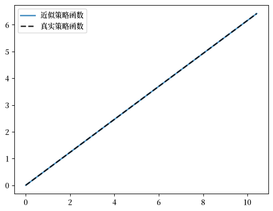
拟合效果非常好。
max_dev = jnp.max(jnp.abs(c - σ_star(x, model.α, model.β)))
print(f"Maximum absolute deviation: {max_dev:.7}")
Maximum absolute deviation: 2.384186e-06
由于 JIT 编译和向量化,JAX 实现非常快。
with qe.Timer(precision=8):
    c, x = solve_model_time_iter(model, c_init, x_init)
    jax.block_until_ready(c)
0.00622416 seconds elapsed
这种速度来自于:
对整个求解器进行 JIT 编译
通过 Coleman-Reffett 算子中的
vmap进行向量化使用
jax.lax.while_loop而非 Python 循环全程使用高效的 JAX 数组操作
70.3. 练习#
练习 70.1
求解具有 CRRA 效用的最优储蓄问题
比较 \(\gamma\) 从上方接近 1 时(例如 1.05、1.1、1.2)的最优策略。
证明当 \(\gamma \to 1\) 时,最优策略收敛到使用对数效用(\(\gamma = 1\))得到的策略。
提示:使用接近 1 的 \(\gamma\) 值以确保内生网格具有相似的覆盖范围,从而使可视化比较更容易。
解答 练习 70.1
我们需要创建一个能够处理 CRRA 效用的 Coleman-Reffett 算子和求解器版本。
关键在于将效用函数用 \(\gamma\) 参数化。
def u_crra(c, γ):
    return (c**(1 - γ) - 1) / (1 - γ)

def u_prime_crra(c, γ):
    return c**(-γ)

def u_prime_inv_crra(x, γ):
    return x**(-1/γ)
现在我们创建一个以 \(\gamma\) 作为参数的 Coleman-Reffett 算子版本。
def K_crra(
        c_in: jnp.ndarray,  # 内生网格上的消费值
        x_in: jnp.ndarray,  # 当前内生网格
        model: Model,       # 模型规格
        γ: float            # CRRA 参数
    ):
    """
    使用 EGM 和 CRRA 效用的 Coleman-Reffett 算子
    """
    # 简化名称
    β, α = model.β, model.α
    s_grid, shocks = model.s_grid, model.shocks

    # 使用内生网格对策略进行线性插值
    σ = lambda x_val: jnp.interp(x_val, x_in, c_in)

    # 定义在单个网格点上计算消费的函数
    def compute_c(s):
        vals = u_prime_crra(σ(f(s, α) * shocks), γ) * f_prime(s, α) * shocks
        return u_prime_inv_crra(β * jnp.mean(vals), γ)

    # 使用 vmap 在网格上向量化
    compute_c_vectorized = jax.vmap(compute_c)
    c_out = compute_c_vectorized(s_grid)

    # 确定对应的内生网格
    x_out = s_grid + c_out  # x_i = s_i + c_i

    return c_out, x_out
我们还需要一个使用该算子的求解器。
@jax.jit
def solve_model_crra(model: Model,
                     c_init: jnp.ndarray,
                     x_init: jnp.ndarray,
                     γ: float,
                     tol: float = 1e-5,
                     max_iter: int = 1000):
    """
    使用带 EGM 和 CRRA 效用的时间迭代求解模型。
    """

    def condition(loop_state):
        i, c, x, error = loop_state
        return (error > tol) & (i < max_iter)

    def body(loop_state):
        i, c, x, error = loop_state
        c_new, x_new = K_crra(c, x, model, γ)
        error = jnp.max(jnp.abs(c_new - c))
        return i + 1, c_new, x_new, error

    # 初始化循环状态
    initial_state = (0, c_init, x_init, tol + 1)

    # 运行循环
    i, c, x, error = jax.lax.while_loop(condition, body, initial_state)

    return c, x
现在我们对 \(\gamma = 1\)(对数效用)以及从上方接近 1 的值进行求解。
γ_values = [1.0, 1.05, 1.1, 1.2]
policies = {}
endogenous_grids = {}

model_crra = create_model()

for γ in γ_values:
    c_init = jnp.copy(model_crra.s_grid)
    x_init = model_crra.s_grid + c_init
    c_gamma, x_gamma = solve_model_crra(model_crra, c_init, x_init, γ)
    jax.block_until_ready(c_gamma)
    policies[γ] = c_gamma
    endogenous_grids[γ] = x_gamma
    print(f"Solved for γ = {γ}")
Solved for γ = 1.0
Solved for γ = 1.05
Solved for γ = 1.1
Solved for γ = 1.2
在各自的内生网格上绘制策略。
fig, ax = plt.subplots()

for γ in γ_values:
    x = endogenous_grids[γ]
    if γ == 1.0:
        ax.plot(x, policies[γ], 'k-', linewidth=2,
                label=f'γ = {γ:.2f} (对数效用)', alpha=0.8)
    else:
        ax.plot(x, policies[γ], label=f'γ = {γ:.2f}', alpha=0.8)

ax.set_xlabel('状态 x')
ax.set_ylabel('消费 σ(x)')
ax.legend()
ax.set_title('最优策略:CRRA 效用接近对数情形')
plt.show()
findfont: Failed to find font weight normal, now using 600.
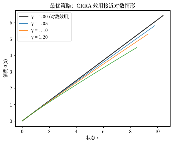
注意,\(\gamma > 1\) 的图形并未覆盖所示的整个 x 轴范围。
这是因为内生网格 \(x = s + \sigma(s)\) 取决于消费策略,而消费策略随 \(\gamma\) 变化。
让我们检查对数效用情形(\(\gamma = 1.0\))与从上方接近的值之间的最大偏差。
for γ in [1.05, 1.1, 1.2]:
    max_diff = jnp.max(jnp.abs(policies[1.0] - policies[γ]))
    print(f"Max difference between γ=1.0 and γ={γ}: {max_diff:.6}")
Max difference between γ=1.0 and γ=1.05: 0.619195
Max difference between γ=1.0 and γ=1.1: 1.13619
Max difference between γ=1.0 and γ=1.2: 1.94591
正如预期,随着 \(\gamma\) 从上方接近 1,差异逐渐减小,这证实了收敛性。