.md .pdf

Contents

Getting Setup for the Workshop

The following steps will help you get all the necessary software needed for the workshop.

Please go through this before the workshop so that you are familiar with:

1. how to open jupyter notebooks, and

2. are comfortable getting access to python.

Step 1: Installing Python (Anaconda)

The Python ecosystem consists of a lot of software packages that bring extended functionality and high productivity straight away.

To manage these packages it is strongly recommended that you install the Anaconda Python Distribution

This enables you to get access to the majority of packages you will need to do your work without any configuration and tracking of software dependencies.

You can download the latest from here or search Anaconda Python and install the Individual Edition.

Please follow the Anaconda Installation Guides and install Python 3.8 on your computer:

macOS

Please use the Anaconda installer guide for macOS

Note

If you have an M1 based mac you will need to install using Rosetta2 emulation. A handy blog post details some additional steps to sort out any possible issues using terminal. Please let me know if you have any issues.

Windows 10

Please use the Anaconda installer guide for Windows

Tip

If you are a Windows user and would like access to the broader linux based tools we have had a lot of success using windows subsystem for linux. This gives you to a lot of powerful tools via terminal based workflows.

Warning

You can add anaconda to your system PATH but it will affect other applications that use python across Windows. Continuum recommend using the Anaconda Prompt provided by the installer.

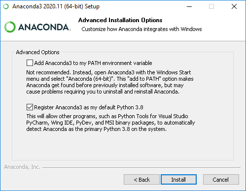
Please leave this box unticked if you are not sure.

Linux

Please use the Anaconda installer guide for Linux

An Anaconda Starter Guide is also available to download.

Step 2: Running Jupyter

Jupyter Notebooks have become a standard tool in the datascience community that marries up:

1. writing code, and

2. writing prose

They are often described as computational narratives.

At the basic level it provides two cells that can be used to write Markdown or Code:

1. A Markdown Cell allows you to write notes, comments, ideas, include figures etc.

2. A Code Cell is for executable code that is connected to a language kernel and fetches the output.

We will be using jupyter notebooks in this workshop, and jupyter comes pre-packaged with anaconda so if you have completed Step 1 you have jupyter on your system.

It also provides a nice interface to start using Python. I do a lot of my exploratory work in Jupyter Notebooks.

Tip

If you get stuck a good first place to look is the Jupyter notebook documentation

Launching Jupyter Notebook

Jupyter is a server that runs on your computer that connects the front-end html based interface with programming language kernels (such as python) to execute code and get results.

Tip

Jupyter Lab is also available. It provides a more comprehensive Integrated Development Environment (IDE). I tend to use jupyter notebooks as they are a simpler interface but there is a lot of development going into Jupyter Lab and you may want to explore using it.

If you haven’t been able to get setup yet you can also try out the Jupyter Notebook in the cloud

Terminal based Workflow (Recommended)

Terminal based workflows can be a very convenient way to launch applications (like jupyter) and run programs.

A GUI based workflow is also available below.

macOS

You can open terminal using:

1. Finder to open Applications/Utilities/Terminal, or

2. Spotlight to search for terminal

Tip

It can be useful to change directory to where the notebook files you are working on are located before launching the jupyter server. This makes accessing your files easier.

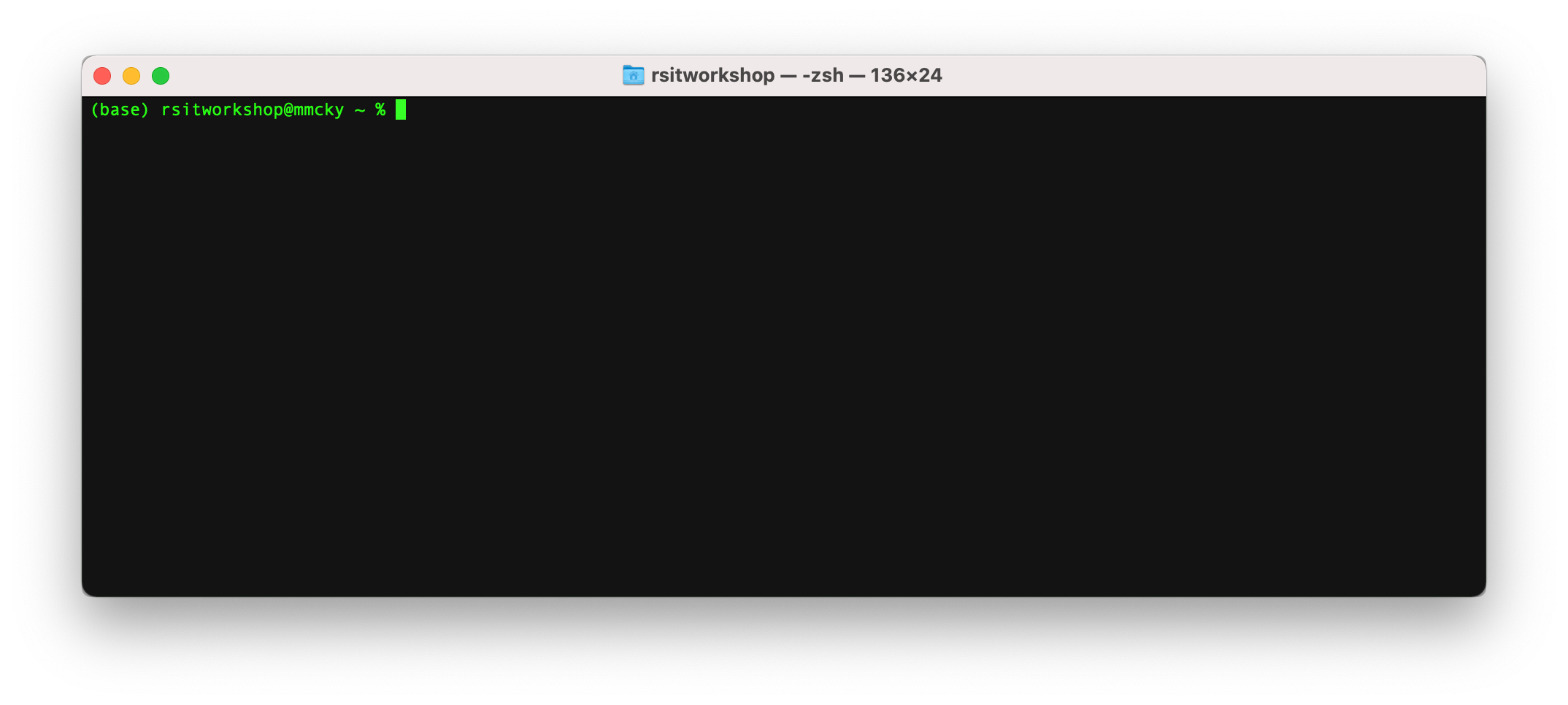
then you can type jupyter notebook to launch a jupyter notebook server:

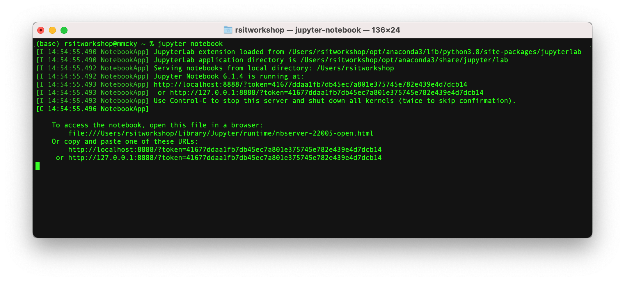
A browser will then open with a running jupyter notebook home page as shown in the next section

Windows 10

The recommended way to open a terminal for Anaconda is to use the Anaconda Prompt provided by the installer. This ensures python is available on your PATH:

Open Start Menu and then open Anaconda3 and click on Anaconda Prompt

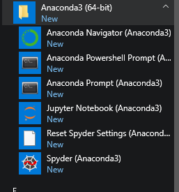
this will open

Tip

It can be useful to change directory to where the notebook files you are working on are located before launching the jupyter server. This makes accessing your files easier.

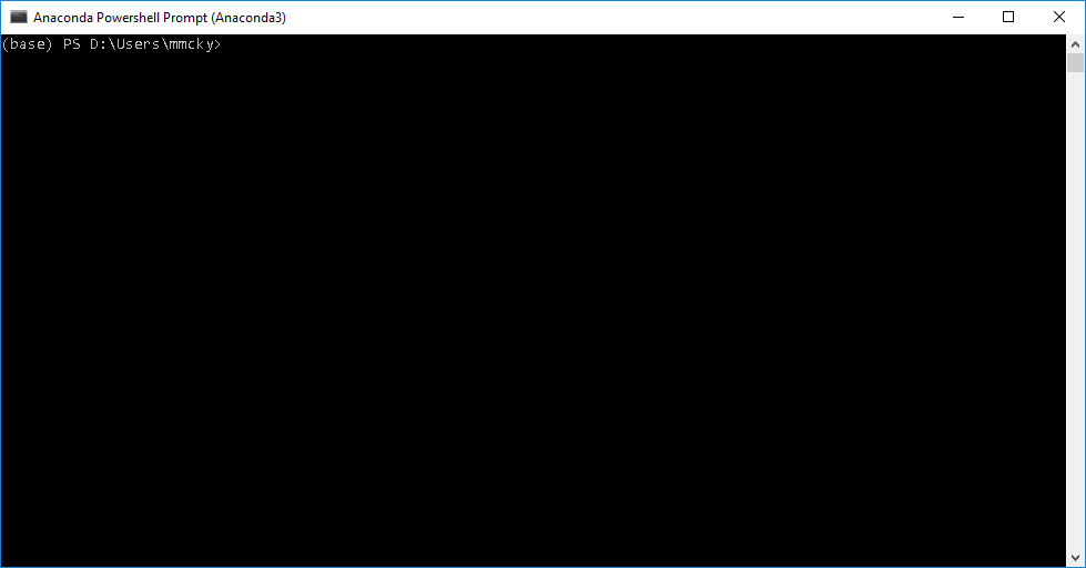
then you can type jupyter notebook to launch a jupyter notebook server:

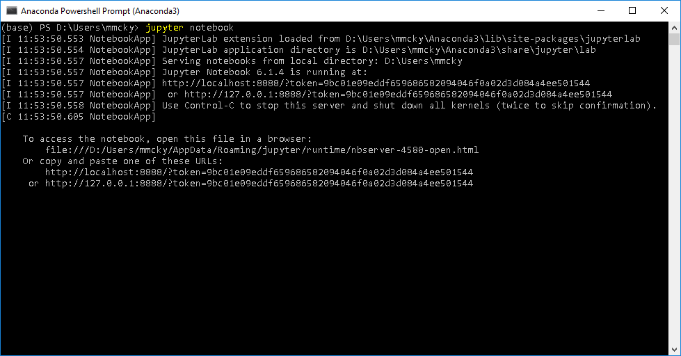
A browser will then open with a running jupyter notebook home page as shown in the next section

Linux

Tip

It can be useful to change directory to where the notebook files you are working on are located before launching the jupyter server. This makes accessing your files easier.

Note

The linux setup is the same as OS X once you open the default terminal application for your linux distribution.

GUI based Workflow

There is a Graphical User Interface (GUI) available for launching Jupyter Notebook or Jupyter Lab provided by Anaconda.

macOS

Jupyter can be opened using a GUI application that comes with Anaconda by:

1. Open Finder and select Applications

2. Click on Anaconda Navigator

The following window will open:

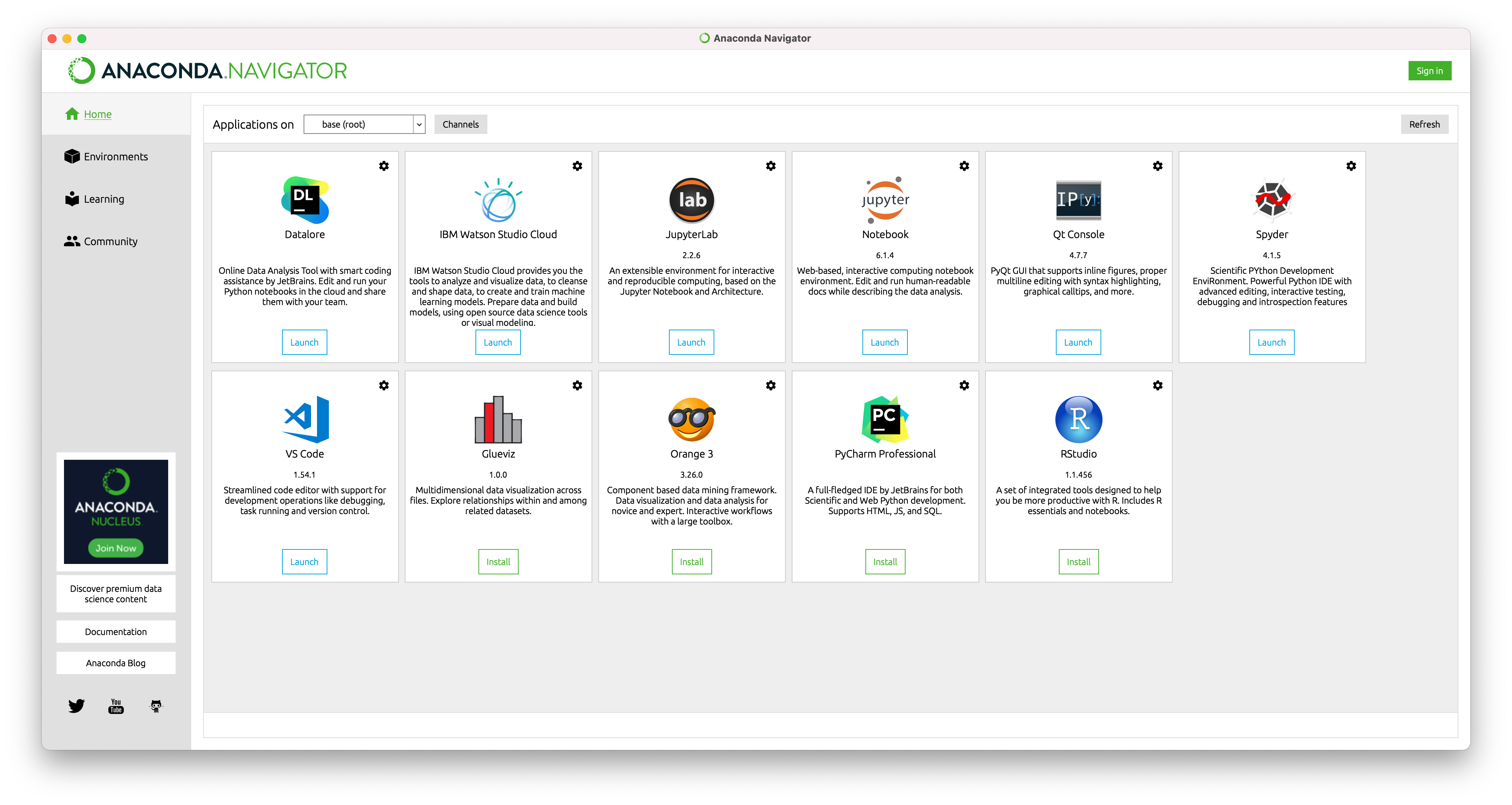
Click on Jupyter Notebook and a browser will then open with a running jupyter notebook home page as shown in the next section.

Windows

Jupyter can be opened using a GUI application that comes with Anaconda by:

1. Click on Start Menu and navigate to Anaconda3

2. Click on Anaconda Navigator

The following window will open:

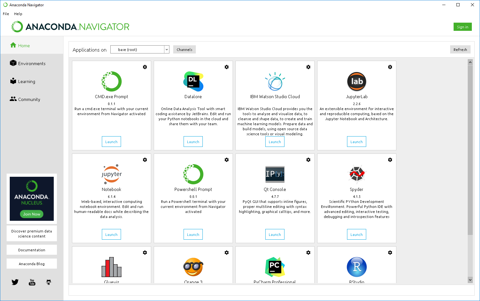
Click on Jupyter Notebook and a browser will then open with a running jupyter notebook home page as shown in the next section.

Linux

If you’re using Linux then I presume you will use terminal based workflows

Anaconda Navigator is available but it largely depends on Linux distribution on how to open the application.

Step 3: Creating / Opening an ipynb file

Once you have the jupyter server running you will see the following in your browser:

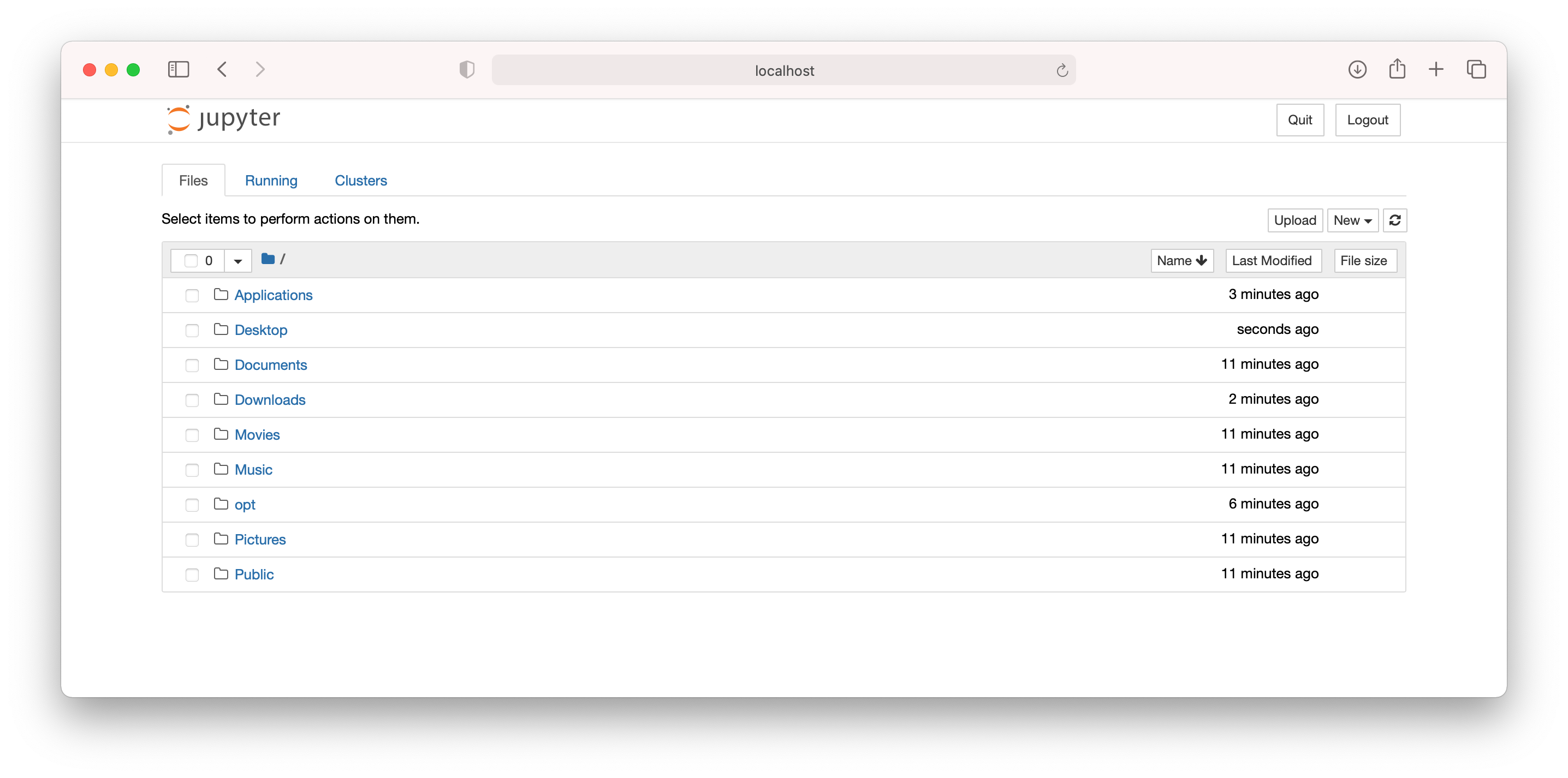
this is a file navigator view so that you can change directory or navigate to a file if you didn’t open the jupyter server in your working directory containing notebooks

Then click on New:

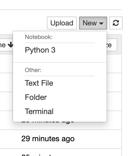
and select Python as your language.

A notebook will open in another tab:

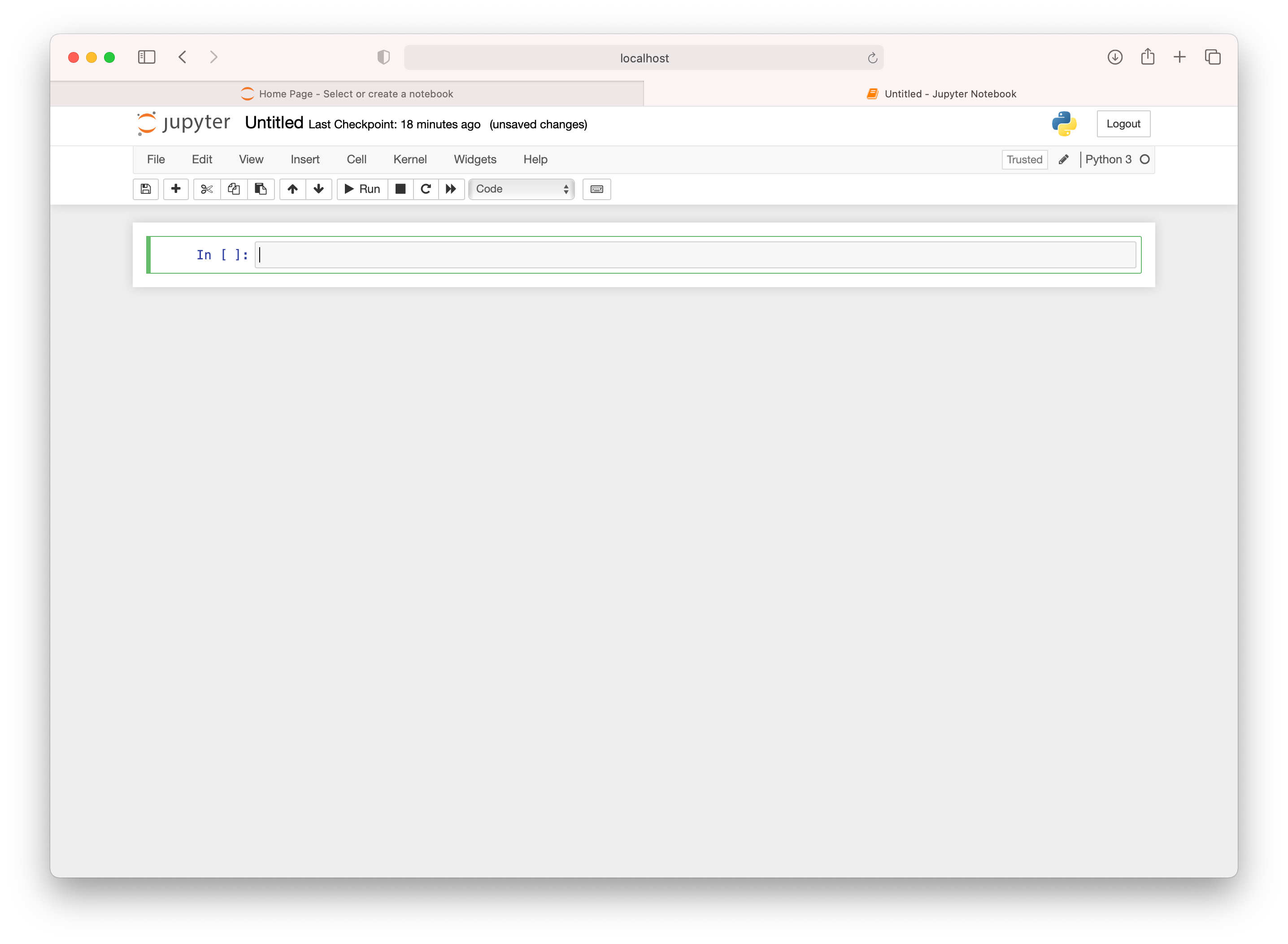
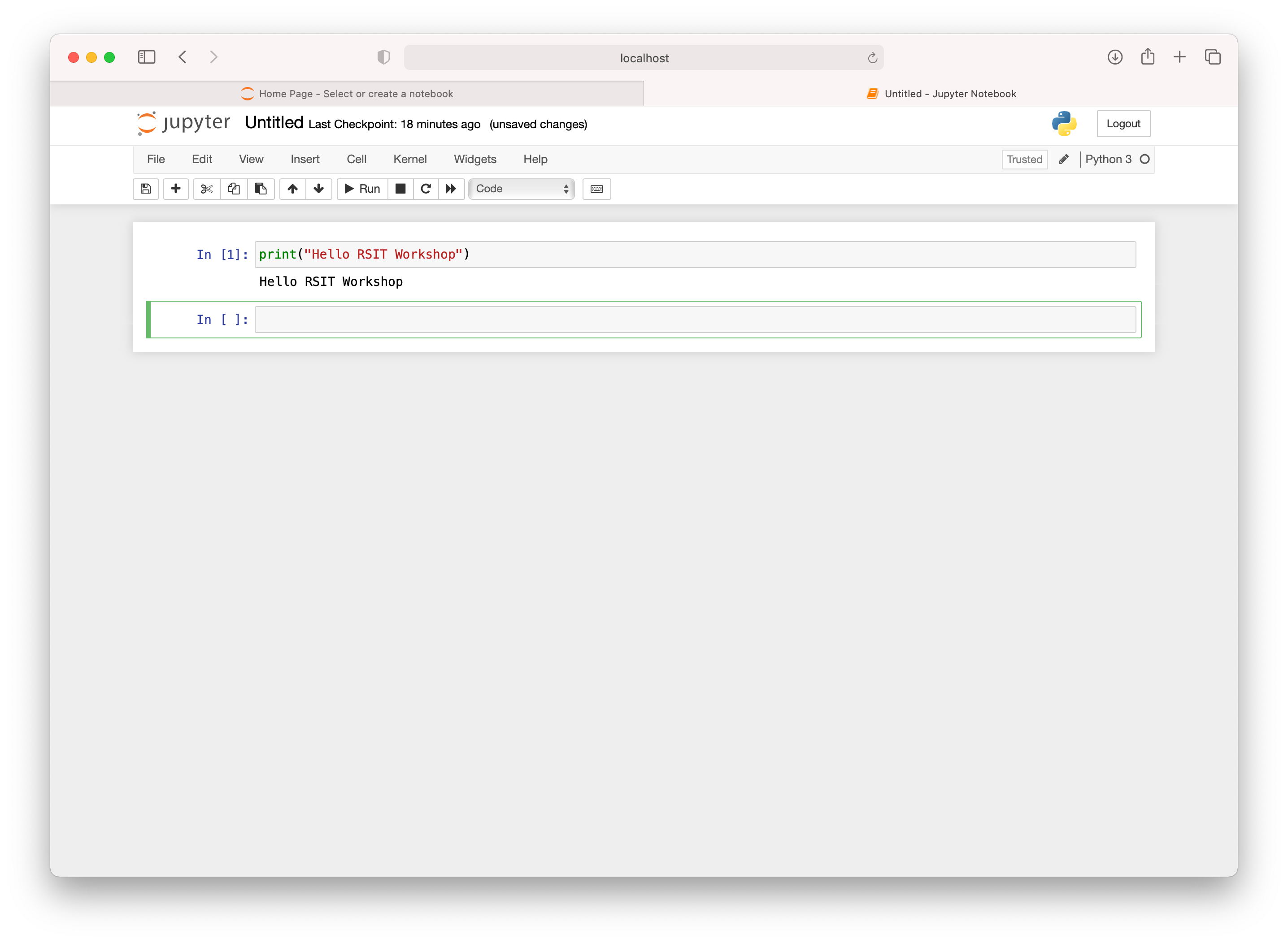
you can then write some python code such as:

print("Hello RSIT Workshop")

and use Command + Enter to execute the code and get the results

Step 4: Exercises

Here are some exercises to help you get started with Jupyter Notebooks and running your own programs and linking you to further documentation to learn more about them.

Tip

Open a Jupyter Notebook and spend some time to have a look around at the menus and interface.

Exercise 6

Go through the Classic Notebook tutorial on the Jupyter website

Have a read through:

1. QuantEcon: Jupyter Notebooks

2. Jupyter notebook documentation

Exercise 7

Open a jupyter notebook document and select New and use python3 (or python) as your language kernel.

Let’s run your first program. Activate the first cell by clicking on it and type:

print("Hello RSIT Workshop")

this should print the string in the output block below the code-cell

now try running:

%matplotlib inline
import matplotlib.pyplot as plt
import numpy as np

x = np.linspace(0, 10, 200)
y = np.sin(x)

plt.plot(x, y, 'b-', linewidth=2)
plt.show()

think through each line and what might be happening. python is fairly readable out of the box.

Exercise 8

Replicate the code in this lecture in your own Jupyter Notebook:

https://python-programming.quantecon.org/python_by_example.html

by stepping through each code block and copying it into your own notebook.

Alternatively, you can also download an ipynb version of the page:

and/or run this lecture in the cloud using the play button

Workflow Tools How will the Workshop work?