10. NumPy#
“让我们说清楚:科学工作与共识毫无关系。共识是政治的事务。相反,科学只需要一个恰好正确的研究者,这意味着他或她的结果可以通过参照现实世界加以验证。在科学中,共识是无关紧要的。重要的是可重复的结果。” —— 迈克尔·克莱顿
除了 Anaconda 中已有的内容外,本讲座还需要以下库:
!pip install quantecon
10.1. 概述#
NumPy 是一个一流的数值编程库
在学术界、金融界和工业界广泛使用。
成熟、快速、稳定,并持续开发中。
在前几讲中,我们已经看到了一些涉及 NumPy 的代码。
在本讲座中,我们将开始对以下内容进行更系统的讨论:
NumPy 数组,以及
NumPy 提供的基本数组处理操作。
(有关备选参考资料,请参阅 NumPy 官方文档。)
我们将使用以下导入语句。
import numpy as np
import random
import quantecon as qe
import matplotlib.pyplot as plt
import matplotlib as mpl  # i18n
import matplotlib.font_manager  # i18n
FONTPATH = "_fonts/SourceHanSerifSC-SemiBold.otf"  # i18n
mpl.font_manager.fontManager.addfont(FONTPATH)  # i18n
import logging  # i18n
logging.getLogger('matplotlib.font_manager').setLevel(logging.ERROR)  # i18n
mpl.rcParams['font.family'] = ['Source Han Serif SC']  # i18n
from mpl_toolkits.mplot3d.axes3d import Axes3D
from matplotlib import cm
10.2. NumPy 数组#
NumPy 解决的核心问题是快速数组处理。
NumPy 定义的最重要结构是一种数组数据类型,正式称为 numpy.ndarray。
NumPy 数组支撑着科学 Python 生态系统的绝大部分。
10.2.1. 基础#
要创建一个只包含零的 NumPy 数组,我们使用 np.zeros
a = np.zeros(3)
a
array([0., 0., 0.])
type(a)
numpy.ndarray
NumPy 数组与原生 Python 列表有些类似,但有以下区别:
数据必须是同质的(所有元素具有相同的类型)。
这些类型必须是 NumPy 提供的数据类型(
dtypes)之一。
这些 dtypes 中最重要的是:
float64:64 位浮点数
int64:64 位整数
bool:8 位真或假
还有用于表示复数、无符号整数等的 dtypes。
在现代机器上,数组的默认 dtype 是 float64
a = np.zeros(3)
type(a[0])
numpy.float64
如果我们想使用整数,可以按如下方式指定:
a = np.zeros(3, dtype=int)
type(a[0])
numpy.int64
10.2.2. 形状与维度#
考虑以下赋值语句
z = np.zeros(10)
这里 z 是一个扁平数组——既不是行向量也不是列向量。
z.shape
(10,)
这里形状元组只有一个元素,即数组的长度(只有一个元素的元组以逗号结尾)。
要给它添加一个额外的维度,我们可以修改 shape 属性
z.shape = (10, 1)   # 将扁平数组转换为列向量(二维)
z
array([[0.],
       [0.],
       [0.],
       [0.],
       [0.],
       [0.],
       [0.],
       [0.],
       [0.],
       [0.]])
z = np.zeros(4)     # 扁平数组
z.shape = (2, 2)    # 二维数组
z
array([[0., 0.],
       [0., 0.]])
在最后一种情况下,要生成 2x2 数组,我们也可以将元组传递给 zeros() 函数,如 z = np.zeros((2, 2))。
10.2.3. 创建数组#
正如我们所见,np.zeros 函数创建一个零数组。
你大概能猜到 np.ones 创建什么。
与之相关的是 np.empty,它在内存中创建数组,以便稍后用数据填充
z = np.empty(3)
z
array([0., 0., 0.])
这里你看到的数字是垃圾值。
(Python 分配了 3 个连续的 64 位内存块,这些内存槽中现有的内容被解释为 float64 值)
要设置等间距数字的网格,使用 np.linspace
z = np.linspace(2, 4, 5) # 从 2 到 4,共 5 个元素
要创建单位矩阵,使用 np.identity 或 np.eye
z = np.identity(2)
z
array([[1., 0.],
       [0., 1.]])
此外,NumPy 数组可以从 Python 列表、元组等使用 np.array 创建
z = np.array([10, 20])                 # 从 Python 列表创建 ndarray
z
array([10, 20])
type(z)
numpy.ndarray
z = np.array((10, 20), dtype=float)    # 这里 'float' 等价于 'np.float64'
z
array([10., 20.])
z = np.array([[1, 2], [3, 4]])         # 从列表的列表创建 2D 数组
z
array([[1, 2],
       [3, 4]])
另请参阅 np.asarray,它执行类似的功能,但不会对已在 NumPy 数组中的数据进行独立复制。
要从包含数值数据的文本文件中读取数组数据,使用 np.loadtxt——详情请参阅文档。
10.2.4. 数组索引#
对于扁平数组,索引与 Python 序列相同:
z = np.linspace(1, 2, 5)
z
array([1. , 1.25, 1.5 , 1.75, 2. ])
z[0]
np.float64(1.0)
z[0:2] # 两个元素,从元素 0 开始
array([1. , 1.25])
z[-1]
np.float64(2.0)
对于 2D 数组,索引语法如下:
z = np.array([[1, 2], [3, 4]])
z
array([[1, 2],
       [3, 4]])
z[0, 0]
np.int64(1)
z[0, 1]
np.int64(2)
以此类推。
列和行可以按如下方式提取
z[0, :]
array([1, 2])
z[:, 1]
array([2, 4])
整数类型的 NumPy 数组也可用于提取元素
z = np.linspace(2, 4, 5)
z
array([2. , 2.5, 3. , 3.5, 4. ])
indices = np.array((0, 2, 3))
z[indices]
array([2. , 3. , 3.5])
最后,dtype 为 bool 的数组可用于提取元素
z
array([2. , 2.5, 3. , 3.5, 4. ])
d = np.array([0, 1, 1, 0, 0], dtype=bool)
d
array([False, True, True, False, False])
z[d]
array([2.5, 3. ])
我们将在下面看到为什么这很有用。
顺便说一句:可以使用切片符号将数组的所有元素设置为一个数字
z = np.empty(3)
z
array([2. , 3. , 3.5])
z[:] = 42
z
array([42., 42., 42.])
10.2.5. 数组方法#
数组有很多有用的方法,所有这些方法都经过精心优化
a = np.array((4, 3, 2, 1))
a
array([4, 3, 2, 1])
a.sort()              # 原地排序 a
a
array([1, 2, 3, 4])
a.sum() # 求和
np.int64(10)
a.mean() # 均值
np.float64(2.5)
a.max() # 最大值
np.int64(4)
a.argmax() # 返回最大元素的索引
np.int64(3)
a.cumsum() # a 元素的累积和
array([ 1, 3, 6, 10])
a.cumprod() # a 元素的累积积
array([ 1, 2, 6, 24])
a.var() # 方差
np.float64(1.25)
a.std() # 标准差
np.float64(1.118033988749895)
a.shape = (2, 2)
a.T                   # 等价于 a.transpose()
array([[1, 3],
       [2, 4]])
另一个值得了解的方法是 searchsorted()。
如果 z 是一个非递减数组,那么 z.searchsorted(a) 返回 z 中第一个 >= a 的元素的索引
z = np.linspace(2, 4, 5)
z
array([2. , 2.5, 3. , 3.5, 4. ])
z.searchsorted(2.2)
np.int64(1)
10.3. 算术运算#
运算符 +、-、*、/ 和 ** 都对数组逐元素作用
a = np.array([1, 2, 3, 4])
b = np.array([5, 6, 7, 8])
a + b
array([ 6, 8, 10, 12])
a * b
array([ 5, 12, 21, 32])
我们可以向每个元素加一个标量,如下所示
a + 10
array([11, 12, 13, 14])
标量乘法类似
a * 10
array([10, 20, 30, 40])
二维数组遵循相同的一般规则
A = np.ones((2, 2))
B = np.ones((2, 2))
A + B
array([[2., 2.],
       [2., 2.]])
A + 10
array([[11., 11.],
       [11., 11.]])
A * B
array([[1., 1.],
       [1., 1.]])
特别地,A * B 不是矩阵乘积,而是逐元素乘积。
10.4. 矩阵乘法#
我们使用 @ 符号进行矩阵乘法,如下所示:
A = np.ones((2, 2))
B = np.ones((2, 2))
A @ B
array([[2., 2.],
       [2., 2.]])
该语法也适用于扁平数组——NumPy 会对你的意图做出合理猜测:
A @ (0, 1)
array([1., 1.])
由于我们是右乘,元组被视为列向量。
10.5. 广播#
(本节扩展了 Jake VanderPlas 提供的关于广播的精彩讨论。)
Note
广播是 NumPy 非常重要的特性。同时,高级广播相对复杂,以下的一些细节在第一次阅读时可以略读。
在逐元素操作中,数组可能没有相同的形状。
当发生这种情况时,NumPy 将在可能的情况下自动将数组扩展为相同的形状。
NumPy 中这种有用(但有时令人困惑)的特性称为广播。
广播的价值在于:
可以避免
for循环,这有助于数值代码快速运行,以及广播可以让我们在不实际在内存中创建某些维度的情况下对数组执行操作,这在数组很大时非常重要。
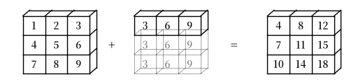
例如,假设 a 是一个 \(3 \times 3\) 数组(a -> (3, 3)),而 b 是一个有三个元素的扁平数组(b -> (3,))。
当将它们相加时,NumPy 将自动将 b -> (3,) 扩展为 b -> (3, 3)。
逐元素加法将产生一个 \(3 \times 3\) 数组
a = np.array(
        [[1, 2, 3],
         [4, 5, 6],
         [7, 8, 9]])
b = np.array([3, 6, 9])

a + b
array([[ 4,  8, 12],
       [ 7, 11, 15],
       [10, 14, 18]])
以下是该广播操作的可视化表示:
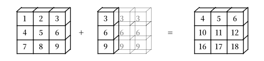
那么 b -> (3, 1) 怎么样?
在这种情况下,NumPy 将自动将 b -> (3, 1) 扩展为 b -> (3, 3)。
逐元素加法将产生一个 \(3 \times 3\) 矩阵
b.shape = (3, 1)

a + b
array([[ 4,  5,  6],
       [10, 11, 12],
       [16, 17, 18]])
以下是该广播操作的可视化表示:
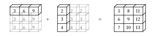
在某些情况下,两个操作数都会被扩展。
当我们有 a -> (3,) 和 b -> (3, 1) 时,a 将被扩展为 a -> (3, 3),b 将被扩展为 b -> (3, 3)。
在这种情况下,逐元素加法将产生一个 \(3 \times 3\) 矩阵
a = np.array([3, 6, 9])
b = np.array([2, 3, 4])
b.shape = (3, 1)

a + b
array([[ 5,  8, 11],
       [ 6,  9, 12],
       [ 7, 10, 13]])
以下是该广播操作的可视化表示:
虽然广播非常有用,但有时可能会令人困惑。
例如,让我们尝试将 a -> (3, 2) 和 b -> (3,) 相加。
a = np.array(
      [[1, 2],
       [4, 5],
       [7, 8]])
b = np.array([3, 6, 9])

a + b
---------------------------------------------------------------------------
ValueError                                Traceback (most recent call last)
Cell In[62], line 7
      3        [4, 5],
      4        [7, 8]])
      5 b = np.array([3, 6, 9])
      6
----> 7 a + b

ValueError: operands could not be broadcast together with shapes (3,2) (3,)
ValueError 告诉我们操作数无法一起广播。
以下是一个可视化表示,说明为什么该广播无法执行:
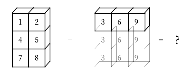
我们可以看到 NumPy 无法将数组扩展为相同的大小。
这是因为当 b 从 b -> (3,) 扩展到 b -> (3, 3) 时,NumPy 无法将 b 与 a -> (3, 2) 匹配。
当我们移动到更高维度时,情况会变得更加复杂。
为了帮助我们理解,可以使用以下规则列表:
第一步:当两个数组的维度不匹配时,NumPy 将通过在现有维度左侧添加维度来扩展维度较少的那个。
例如,如果
a -> (3, 3)且b -> (3,),则广播将在左侧添加一个维度,使得b -> (1, 3);如果
a -> (2, 2, 2)且b -> (2, 2),则广播将在左侧添加一个维度,使得b -> (1, 2, 2);如果
a -> (3, 2, 2)且b -> (2,),则广播将在左侧添加两个维度,使得b -> (1, 1, 2)(你也可以将此过程视为经历了第一步两次)。
第二步:当两个数组具有相同维度但不同形状时,NumPy 将尝试扩展形状索引为 1 的维度。
例如,如果
a -> (1, 3)且b -> (3, 1),则广播将扩展a和b中形状为 1 的维度,使得a -> (3, 3)且b -> (3, 3);如果
a -> (2, 2, 2)且b -> (1, 2, 2),则广播将扩展b的第一个维度,使得b -> (2, 2, 2);如果
a -> (3, 2, 2)且b -> (1, 1, 2),则广播将在所有形状为 1 的维度上扩展b,使得b -> (3, 2, 2)。
第三步:经过第一步和第二步后,如果两个数组仍然不匹配,将引发
ValueError。例如,假设a -> (2, 2, 3)且b -> (2, 2)通过第一步,
b将被扩展为b -> (1, 2, 2);通过第二步,
b将被扩展为b -> (2, 2, 2);我们可以看到经过前两步后它们仍然不匹配。因此,将引发
ValueError
10.6. 可变性与数组复制#
NumPy 数组是可变数据类型,类似于 Python 列表。
换句话说,它们的内容可以在初始化后在内存中被更改(变异)。
这很方便,但与 Python 的命名和引用模型结合时,可能会导致 NumPy 初学者犯错误。
在本节中,我们回顾一些关键问题。
10.6.1. 可变性#
我们在上面已经看到了可变性的例子。
以下是 NumPy 数组变异的另一个例子
a = np.array([42, 44])
a
array([42, 44])
a[-1] = 0  # 将最后一个元素改为 0
a
array([42, 0])
可变性导致以下行为(这可能会让 MATLAB 程序员感到震惊……)
rng = np.random.default_rng()
a = rng.standard_normal(3)
a
array([ 0.78322284, 0.56285284, -0.37223772])
b = a
b[0] = 0.0
a
array([ 0. , 0.56285284, -0.37223772])
发生的情况是我们通过修改 b 改变了 a。
名称 b 绑定到 a,成为该数组的另一个引用(Python 赋值模型在 课程后面 有更详细的描述)。
因此,它有同等权利对该数组进行更改。
这实际上是最合理的默认行为!
这意味着我们只传递数据指针,而不是复制数据。
复制在速度和内存方面都是昂贵的。
10.6.2. 复制数组#
当然,在需要时可以使 b 成为 a 的独立副本。
这可以使用 np.copy 来完成
a = rng.standard_normal(3)
a
array([-0.41336699, 1.66264647, -0.69649387])
b = np.copy(a)
b
array([-0.41336699, 1.66264647, -0.69649387])
现在 b 是一个独立副本(称为深拷贝)
b[:] = 1
b
array([1., 1., 1.])
a
array([-0.41336699, 1.66264647, -0.69649387])
注意对 b 的更改没有影响 a。
10.7. 其他功能#
让我们来看看 NumPy 的其他一些有用功能。
10.7.1. 通用函数#
NumPy 提供了标准函数 log、exp、sin 等的版本,这些版本对数组逐元素作用
z = np.array([1, 2, 3])
np.sin(z)
array([0.84147098, 0.90929743, 0.14112001])
这消除了对显式逐元素循环的需求,例如
n = len(z)
y = np.empty(n)
for i in range(n):
    y[i] = np.sin(z[i])
因为它们对数组逐元素作用,这些函数有时被称为向量化函数。
在 NumPy 的术语中,它们也被称为 ufuncs,或通用函数。
如上所述,常规算术运算(+、* 等)也是逐元素工作的,将这些与 ufuncs 结合起来,可以得到非常大量的快速逐元素函数。
z
array([1, 2, 3])
(1 / np.sqrt(2 * np.pi)) * np.exp(- 0.5 * z**2)
array([0.24197072, 0.05399097, 0.00443185])
并非所有用户自定义函数都会逐元素作用。
例如,将下面定义的函数 f 传递给 NumPy 数组会导致 ValueError
def f(x):
    return 1 if x > 0 else 0
NumPy 函数 np.where 提供了一个向量化的替代方案:
x = rng.standard_normal(4)
x
array([-1.02842863, 1.0392059 , -1.30018299, -1.21695584])
np.where(x > 0, 1, 0) # 如果 x > 0 为真则插入 1,否则插入 0
array([0, 1, 0, 0])
你也可以使用 np.vectorize 来向量化给定的函数
f = np.vectorize(f)
f(x)                # 传递与前一个例子中相同的向量 x
array([0, 1, 0, 0])
但是,这种方法并不总能获得与精心设计的向量化函数相同的速度。
(稍后我们将看到 JAX 有一个强大的 np.vectorize 版本,通常确实可以生成高效的代码。)
10.7.2. 比较#
通常,对数组的比较是逐元素进行的
z = np.array([2, 3])
y = np.array([2, 3])
z == y
array([ True, True])
y[0] = 5
z == y
array([False, True])
z != y
array([ True, False])
>、<、>= 和 <= 的情况类似。
我们也可以与标量进行比较
z = np.linspace(0, 10, 5)
z
array([ 0. , 2.5, 5. , 7.5, 10. ])
z > 3
array([False, False, True, True, True])
这对于条件提取特别有用
b = z > 3
b
array([False, False, True, True, True])
z[b]
array([ 5. , 7.5, 10. ])
当然,我们可以——而且经常——在一个步骤中完成这些操作
z[z > 3]
array([ 5. , 7.5, 10. ])
10.7.3. 子包#
NumPy 通过其子包提供了一些与科学编程相关的附加功能。
我们已经看到了如何使用 NumPy 的 随机 Generator 生成随机变量。
z = rng.standard_normal(10000)  # 生成标准正态随机数
y = rng.binomial(10, 0.5, size=1000)    # 从 Bin(10, 0.5) 中抽取 1000 个样本
y.mean()
np.float64(4.92)
另一个常用的子包是 np.linalg
A = np.array([[1, 2], [3, 4]])

np.linalg.det(A)           # 计算行列式
np.float64(-2.0000000000000004)
np.linalg.inv(A) # 计算逆矩阵
array([[-2. ,  1. ],
       [ 1.5, -0.5]])
这些功能的大部分也可在 SciPy 中找到,SciPy 是建立在 NumPy 之上的模块集合。
我们将在 不久后 更详细地介绍 SciPy 版本。
有关 NumPy 中可用内容的完整列表,请参阅 此文档。
10.7.4. 隐式多线程#
之前我们讨论了通过多线程实现并行化的概念。
NumPy 在其大部分编译代码中尝试实现多线程。
让我们看一个例子来观察这一点。
下面这段代码计算大量随机生成矩阵的特征值。
运行需要几秒钟。
n = 20
m = 1000
for i in range(n):
    X = rng.standard_normal((m, m))
    λ = np.linalg.eigvals(X)
现在,让我们看看这段代码运行时机器上 htop 系统监视器的输出:
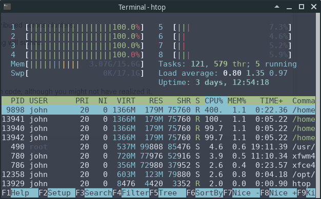
我们可以看到 8 个 CPU 中有 4 个在全速运行。
这是因为 NumPy 的 eigvals 例程巧妙地将任务分割并分发到不同的线程。
10.8. 练习#
Exercise 10.1
考虑多项式表达式
之前,你编写了一个简单函数 p(x, coeff) 来求解 (10.1),但没有考虑效率。
现在编写一个执行相同任务的新函数,但使用 NumPy 数组和数组操作进行计算,而不是任何形式的 Python 循环。
(这样的功能已经在 np.poly1d 中实现,但为了练习目的,请不要使用该类)
Hint
使用 np.cumprod()
Solution
这段代码完成了任务
def p(x, coef):
    X = np.ones_like(coef)
    X[1:] = x
    y = np.cumprod(X)   # y = [1, x, x**2,...]
    return coef @ y
让我们测试它
x = 2
coef = np.linspace(2, 4, 3)
print(coef)
print(p(x, coef))
# 作为对比
q = np.poly1d(np.flip(coef))
print(q(x))
[2. 3. 4.]
24.0
24.0
Exercise 10.2
设 q 是长度为 n 且 q.sum() == 1 的 NumPy 数组。
假设 q 表示一个概率质量函数。
我们希望生成一个离散随机变量 \(x\),使得 \(\mathbb P\{x = i\} = q_i\)。
换句话说,x 取 range(len(q)) 中的值,且 x = i 的概率为 q[i]。
标准(逆变换)算法如下:
将单位区间 \([0, 1]\) 分成 \(n\) 个子区间 \(I_0, I_1, \ldots, I_{n-1}\),使得 \(I_i\) 的长度为 \(q_i\)。
在 \([0, 1]\) 上抽取一个均匀随机变量 \(U\),返回满足 \(U \in I_i\) 的 \(i\)。
抽到 \(i\) 的概率是 \(I_i\) 的长度,等于 \(q_i\)。
我们可以如下实现该算法
from random import uniform

def sample(q):
    a = 0.0
    U = uniform(0, 1)
    for i in range(len(q)):
        if a < U <= a + q[i]:
            return i
        a = a + q[i]
如果你不明白这是如何工作的,试着通过一个简单的例子来理解流程,例如 q = [0.25, 0.75]。
在纸上画出区间会有帮助。
你的练习是使用 NumPy 加速它,避免显式循环
Hint
使用 np.searchsorted 和 np.cumsum
如果可以的话,将功能实现为名为 DiscreteRV 的类,其中
类的实例数据是概率向量
q该类有一个
draw()方法,根据上述算法返回一个样本
如果可以的话,编写该方法使得 draw(k) 从 q 中返回 k 个样本。
Solution
以下是我们的初始解决方案:
from numpy import cumsum

class DiscreteRV:
    """
    根据给定概率向量 q 生成离散随机变量的抽样数组。
    """

    def __init__(self, q, seed=None):
        """
        参数 q 是一个 NumPy 数组或类似数组,非负且和为 1。

        参数 seed 为底层随机数生成器设置种子;默认 seed=None 时,
        每次运行的抽样结果不可重现。
        """
        self.q = q
        self.Q = cumsum(q)
        self.rng = np.random.default_rng(seed)

    def draw(self, k=1):
        """
        从 q 中返回 k 个样本。对于每次抽样,值 i 以概率 q[i] 返回。
        """
        return self.Q.searchsorted(self.rng.uniform(0, 1, size=k))
逻辑不是很直观,但如果你慢慢阅读,就会理解。
然而,这里有一个问题。
假设在创建 DiscreteRV 实例后修改了 q,例如
q = (0.1, 0.9)
d = DiscreteRV(q)
d.q = (0.5, 0.5)
问题是 Q 不会相应地改变,而 Q 是 draw 方法中使用的数据。
要处理这个问题,一个选项是每次调用 draw 方法时都计算 Q。
但这相对于一次性计算 Q 来说效率较低。
一个更好的选项是使用描述符。
quantecon 库中使用描述符的解决方案,其行为符合我们的要求,可以在这里找到。
Exercise 10.3
回顾我们之前关于经验累积分布函数的讨论。
你的任务是:
使用 NumPy 使
__call__方法更高效。添加一个在 \([a, b]\) 上绘制经验累积分布函数的方法,其中 \(a\) 和 \(b\) 是方法参数。
Solution
下面给出了一个示例解决方案。
本质上,我们只是取了来自 QuantEcon 的这段代码并添加了绘图方法
"""
修改 QuantEcon 的 ecdf.py 以添加绘图方法

"""

class ECDF:
    """
    给定观测向量的一维经验分布函数。

    Parameters
    ----------
    observations : array_like
        观测数组

    Attributes
    ----------
    observations : array_like
        观测数组

    """

    def __init__(self, observations):
        self.observations = np.asarray(observations)

    def __call__(self, x):
        """
        在 x 处评估经验累积分布函数

        Parameters
        ----------
        x : scalar(float)
            评估经验累积分布函数的 x 值

        Returns
        -------
        scalar(float)
            样本中小于 x 的比例

        """
        return np.mean(self.observations <= x)

    def plot(self, ax, a=None, b=None):
        """
        在区间 [a, b] 上绘制经验累积分布函数。

        Parameters
        ----------
        a : scalar(float), optional(default=None)
            绘图区间的下端点
        b : scalar(float), optional(default=None)
            绘图区间的上端点

        """

        # === 如果未指定 [a, b],则选择合理的区间 === #
        if a is None:
            a = self.observations.min() - self.observations.std()
        if b is None:
            b = self.observations.max() + self.observations.std()

        # === 生成图形 === #
        x_vals = np.linspace(a, b, num=100)
        f = np.vectorize(self.__call__)
        ax.plot(x_vals, f(x_vals))
        plt.show()
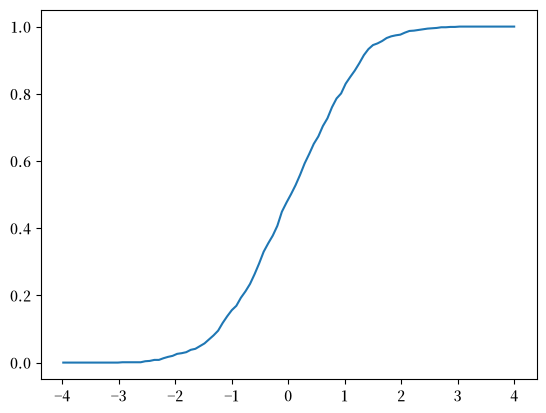
以下是使用示例
fig, ax = plt.subplots()
rng = np.random.default_rng()
X = rng.standard_normal(1000)
F = ECDF(X)
F.plot(ax)
Exercise 10.4
回顾 NumPy 中的广播可以帮助我们在不使用 for 循环的情况下对不同维度的数组执行逐元素操作。
在本练习中,尝试使用 for 循环来复现以下广播操作的结果。
第 1 部分:尝试使用 for 循环复现以下简单示例,并将你的结果与下面的广播操作进行比较。
rng = np.random.default_rng(123)
x = rng.standard_normal((4, 4))
y = rng.standard_normal(4)
A = x / y
以下是输出结果
print(A)
第 2 部分:继续复现以下广播操作的结果。同时,比较广播和你实现的 for 循环的速度。
对于本练习的这一部分,你可以使用 quantecon 库中的 qe.Timer() 上下文管理器来计时执行。
让我们确保已安装该库。
!pip install quantecon
现在我们可以导入 quantecon 包。
rng = np.random.default_rng(123)
x = rng.standard_normal((1000, 100, 100))
y = rng.standard_normal(100)

with qe.Timer("广播操作"):
    B = x / y
广播操作: 0.0116 seconds elapsed
以下是输出结果
print(B)
Solution
第 1 部分解答
rng = np.random.default_rng(123)
x = rng.standard_normal((4, 4))
y = rng.standard_normal(4)

C = np.empty_like(x)
n = len(x)
for i in range(n):
    for j in range(n):
        C[i, j] = x[i, j] / y[j]
比较结果以检查你的答案
print(C)
你也可以使用 array_equal() 来检查你的答案
print(np.array_equal(A, C))
True
第 2 部分解答
rng = np.random.default_rng(123)
x = rng.standard_normal((1000, 100, 100))
y = rng.standard_normal(100)

with qe.Timer("For 循环操作"):
    D = np.empty_like(x)
    d1, d2, d3 = x.shape
    for i in range(d1):
        for j in range(d2):
            for k in range(d3):
                D[i, j, k] = x[i, j, k] / y[k]
For 循环操作: 3.8150 seconds elapsed
注意 for 循环比广播操作花费的时间长得多。
比较结果以检查你的答案
print(D)
print(np.array_equal(B, D))
True