16. 特征值和特征向量#

16.1. 概述#

特征值和特征向量是线性代数中一个相对高级的话题。

同时，这些概念在以下领域非常有用：

经济建模（尤其是动态模型！）
统计学
应用数学的某些部分
机器学习
以及许多其他科学领域

在本讲座中，我们将解释特征值和特征向量的基础知识，并介绍诺伊曼级数引理。

我们假设学生已经熟悉矩阵，并理解矩阵代数的基础知识。

我们将使用以下导入：

import matplotlib.pyplot as plt
import numpy as np
from numpy.linalg import matrix_power
from matplotlib.lines import Line2D
from matplotlib.patches import FancyArrowPatch
from mpl_toolkits.mplot3d import proj3d

import matplotlib as mpl
FONTPATH = "fonts/SourceHanSerifSC-SemiBold.otf"
mpl.font_manager.fontManager.addfont(FONTPATH)
plt.rcParams['font.family'] = ['Source Han Serif SC']

16.2. 矩阵作为变换#

让我们从讨论一个关于矩阵的重要概念开始。

16.2.1. 将向量映射到向量#

有两种思考矩阵的方式：

将矩阵视为一个矩形的数字集合。
将矩阵视为一个将向量转换为新向量的映射（即函数）。

为了理解第二种观点，假设我们将一个 $n \times m$ 矩阵 $A$ 与一个 $m \times 1$ 列向量 $x$ 相乘，得到一个 $n \times 1$ 列向量 $y$ ：

A x = y

如果我们固定 $A$ 并考虑不同的 $x$ ，我们可以将 $A$ 理解为一个将 $x$ 转换为 $A x$ 的映射。

因为 $A$ 是 $n \times m$ 的，所以它将 $m$ 维向量转换为 $n$ 维向量。

我们可以正式地将此写作 $A : R^{m} \to R^{n}$ 。

你可能会说，如果 $A$ 是一个函数，那么我们应该写成 $A (x) = y$ 而不是 $A x = y$ ，但后者的表示方法更为常见。

16.2.2. 方阵#

让我们将讨论限制在方阵上。

在上述讨论中，这意味着 $m = n$ ，则 $A$ 将 $R^{n}$ 映射到自身。

这表示 $A$ 是一个 $n \times n$ 矩阵，它将 $R^{n}$ 中的向量 $x$ 映射（或”变换”）为同样在 $R^{n}$ 中的新向量 $y = A x$ 。

以下是一个例子

Example 16.1

\begin{array}{r} [\begin{array}{c} 2 & 1 \\ - 1 & 1 \end{array}] [\begin{array}{c} 1 \\ 3 \end{array}] = [\begin{array}{c} 5 \\ 2 \end{array}] \end{array}

在这里，矩阵

\begin{array}{r} A = [\begin{array}{c} 2 & 1 \\ - 1 & 1 \end{array}] \end{array}

将向量 $x = [\begin{matrix} 1 \\ 3 \end{matrix}]$ 变换为向量 $y = [\begin{matrix} 5 \\ 2 \end{matrix}]$ 。

让我们用 Python 来可视化这个过程：

A = np.array([[2,  1],
              [-1, 1]])

from math import sqrt

fig, ax = plt.subplots()
# 设置坐标轴通过原点

for spine in ['left', 'bottom']:
    ax.spines[spine].set_position('zero')
for spine in ['right', 'top']:
    ax.spines[spine].set_color('none')

ax.set(xlim=(-2, 6), ylim=(-2, 4), aspect=1)

vecs = ((1, 3), (5, 2))
c = ['r', 'black']
for i, v in enumerate(vecs):
    ax.annotate('', xy=v, xytext=(0, 0),
                arrowprops=dict(color=c[i],
                shrink=0,
                alpha=0.7,
                width=0.5))

ax.text(0.2 + 1, 0.2 + 3, 'x=$(1,3)$')
ax.text(0.2 + 5, 0.2 + 2, 'Ax=$(5,2)$')

ax.annotate('', xy=(sqrt(10/29) * 5, sqrt(10/29) * 2), xytext=(0, 0),
            arrowprops=dict(color='purple',
                            shrink=0,
                            alpha=0.7,
                            width=0.5))

ax.annotate('', xy=(1, 2/5), xytext=(1/3, 1),
            arrowprops={'arrowstyle': '->',
                        'connectionstyle': 'arc3,rad=-0.3'},
            horizontalalignment='center')
ax.text(0.8, 0.8, f'θ', fontsize=14)

plt.show()

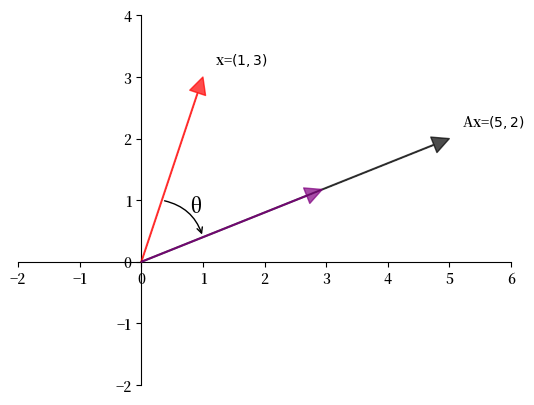
_images/1e9859dab1bf3855d12e6d196363de624a7da34b6c3d53305fb1dab7e8b22bb7.png

我们可以这样理解 $A$ ：

首先将 $x$ 旋转某个角度 $θ$ ，然后
将其缩放某个标量 $γ$ 以获得 $x$ 的像 $y$ 。

16.3. 变换类型#

让我们来检查一些可以用矩阵执行的标准变换。

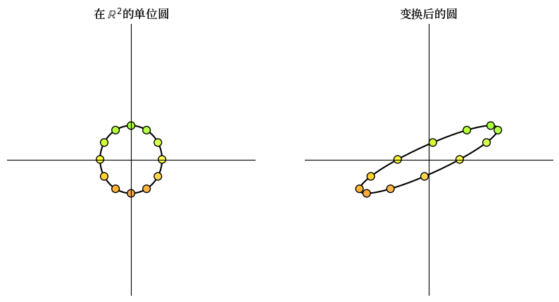
下面我们通过将向量视为点而不是箭头来可视化变换。

我们将给定一个矩阵并观察它如何变换

一个点阵网格和
位于 $R^{2}$ 中单位圆上的一组点。

为了构建这些变换，我们将使用两个函数，称为 grid_transform 和 circle_transform。

这些函数中的每一个都可视化一个特定的 $2 \times 2$ 矩阵 $A$ 的作用。

Show source Hide code cell source

def colorizer(x, y):
    r = min(1, 1-y/3)
    g = min(1, 1+y/3)
    b = 1/4 + x/16
    return (r, g, b)


def grid_transform(A=np.array([[1, -1], [1, 1]])):
    xvals = np.linspace(-4, 4, 9)
    yvals = np.linspace(-3, 3, 7)
    xygrid = np.column_stack([[x, y] for x in xvals for y in yvals])
    uvgrid = A @ xygrid

    colors = list(map(colorizer, xygrid[0], xygrid[1]))

    fig, ax = plt.subplots(1, 2, figsize=(10, 5))

    for axes in ax:
        axes.set(xlim=(-11, 11), ylim=(-11, 11))
        axes.set_xticks([])
        axes.set_yticks([])
        for spine in ['left', 'bottom']:
            axes.spines[spine].set_position('zero')
        for spine in ['right', 'top']:
            axes.spines[spine].set_color('none')

    # 绘制x-y格点
    ax[0].scatter(xygrid[0], xygrid[1], s=36, c=colors, edgecolor="none")
    # ax[0].grid(True)
    # ax[0].axis("equal")
    ax[0].set_title(r"点 $x_1, x_2, \cdots, x_k$")

    # 绘制变换的格点
    ax[1].scatter(uvgrid[0], uvgrid[1], s=36, c=colors, edgecolor="none")
    # ax[1].grid(True)
    # ax[1].axis("equal")
    ax[1].set_title(r"点 $Ax_1, Ax_2, \cdots, Ax_k$")

    plt.show()


def circle_transform(A=np.array([[-1, 2], [0, 1]])):

    fig, ax = plt.subplots(1, 2, figsize=(10, 5))

    for axes in ax:
        axes.set(xlim=(-4, 4), ylim=(-4, 4))
        axes.set_xticks([])
        axes.set_yticks([])
        for spine in ['left', 'bottom']:
            axes.spines[spine].set_position('zero')
        for spine in ['right', 'top']:
            axes.spines[spine].set_color('none')

    θ = np.linspace(0, 2 * np.pi, 150)
    r = 1

    θ_1 = np.empty(12)
    for i in range(12):
        θ_1[i] = 2 * np.pi * (i/12)

    x = r * np.cos(θ)
    y = r * np.sin(θ)
    a = r * np.cos(θ_1)
    b = r * np.sin(θ_1)
    a_1 = a.reshape(1, -1)
    b_1 = b.reshape(1, -1)
    colors = list(map(colorizer, a, b))
    ax[0].plot(x, y, color='black', zorder=1)
    ax[0].scatter(a_1, b_1, c=colors, alpha=1, s=60,
                  edgecolors='black', zorder=2)
    ax[0].set_title(r"在 $\mathbb{R}^2$的单位圆")

    x1 = x.reshape(1, -1)
    y1 = y.reshape(1, -1)
    ab = np.concatenate((a_1, b_1), axis=0)
    transformed_ab = A @ ab
    transformed_circle_input = np.concatenate((x1, y1), axis=0)
    transformed_circle = A @ transformed_circle_input
    ax[1].plot(transformed_circle[0, :],
               transformed_circle[1, :], color='black', zorder=1)
    ax[1].scatter(transformed_ab[0, :], transformed_ab[1:,],
                  color=colors, alpha=1, s=60, edgecolors='black', zorder=2)
    ax[1].set_title("变换后的圆")

    plt.show()

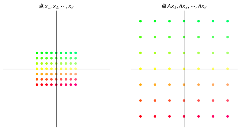
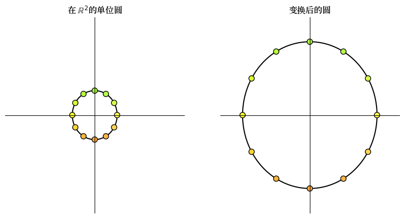
16.3.1. 缩放#

类似

\begin{array}{r} [\begin{array}{c} α & 0 \\ 0 & β \end{array}] \end{array}

的矩阵沿 x 轴将向量缩放 $α$ 倍，沿 y 轴缩放 $β$ 倍。

这里我们举一个简单的例子，其中 $α = β = 3$ 。

A = np.array([[3, 0],  # 在两个方向放大三倍
              [0, 3]])
grid_transform(A)
circle_transform(A)

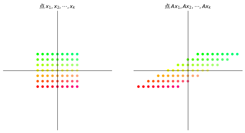
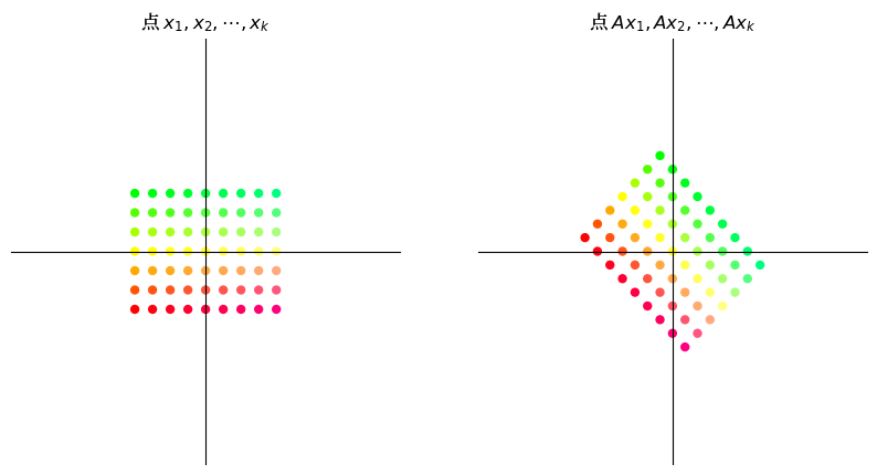
_images/174561a7dc3f858fe01b7a469c91c2b37f2c09b667c22c046858306e58c01c63.png

_images/92029e0ac1c471d423d3bb6ca48b7aaca435a416b46da96fadc5fa8920519507.png

16.3.2. 剪切#

类似

\begin{array}{r} [\begin{array}{c} 1 & λ \\ 0 & 1 \end{array}] \end{array}

的”剪切”矩阵沿 x 轴拉伸向量，拉伸量与点的 y 坐标成比例。

A = np.array([[1, 2],     # 沿x-轴进行剪切
              [0, 1]])
grid_transform(A)
circle_transform(A)

_images/cc2c0de5712d4d6a1128a4bfb214c2eaad5693e06d8d9413f823ab6051aa93b1.png

_images/bd01fb674e18701d5520015468fae97b1b937761b48c0c817742942f063296cc.png

16.3.3. 旋转#

类似

\begin{array}{r} [\begin{array}{c} \cos θ & \sin θ \\ - \sin θ & \cos θ \end{array}] \end{array}

的矩阵被称为 旋转矩阵 。

这个矩阵将向量顺时针旋转角度 $θ$ 。

θ = np.pi/4  # 顺时针旋转45度
A = np.array([[np.cos(θ), np.sin(θ)],
              [-np.sin(θ), np.cos(θ)]])
grid_transform(A)

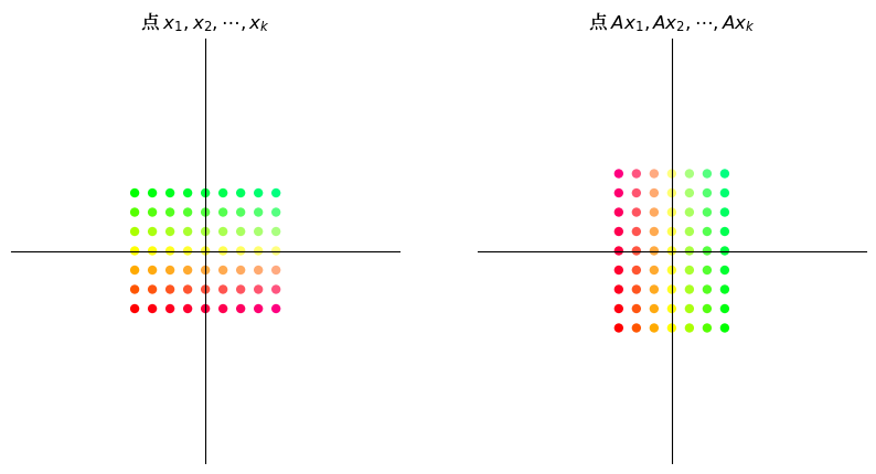
_images/9f0f1f4c3015212db29bd6e6cf267c778bc216efb55fe80e6d577a98f5283a77.png

16.3.4. 置换#

置换矩阵

\begin{array}{r} [\begin{array}{c} 0 & 1 \\ 1 & 0 \end{array}] \end{array}

交换向量的坐标。

A = np.column_stack([[0, 1], [1, 0]])
grid_transform(A)

_images/8c058a575849acd2927818fff2a65acf69e104cca3f620468a80b276c22c1bd2.png

更多常见的变换矩阵示例可以在这里找到。

16.4. 矩阵乘法作为组合#

由于矩阵可以理解为将一个向量转换为另一个向量的函数，我们也可以将函数组合的概念应用于矩阵。

16.4.1. 线性组合#

考虑两个矩阵

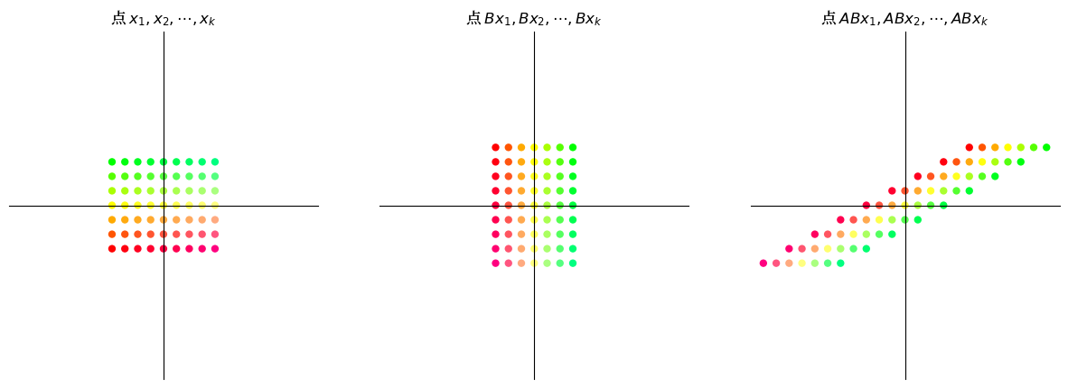
\begin{array}{r} A = [\begin{array}{c} 0 & 1 \\ - 1 & 0 \end{array}] 和 B = [\begin{array}{c} 1 & 2 \\ 0 & 1 \end{array}] \end{array}

当我们尝试对某个 $2 \times 1$ 向量 $x$ 求 $A B x$ 时，输出会是什么？

\begin{array}{r} \underset{A}{\underset{⏟}{[\begin{array}{c} 0 & 1 \\ - 1 & 0 \end{array}]}} \underset{B}{\underset{⏟}{[\begin{array}{c} 1 & 2 \\ 0 & 1 \end{array}]}} \overset{x}{\overset{⏞}{[\begin{array}{c} 1 \\ 3 \end{array}]}} \to \underset{A B}{\underset{⏟}{[\begin{array}{c} 0 & 1 \\ - 1 & - 2 \end{array}]}} \overset{x}{\overset{⏞}{[\begin{array}{c} 1 \\ 3 \end{array}]}} \to \overset{y}{\overset{⏞}{[\begin{array}{c} 3 \\ - 7 \end{array}]}} \end{array}

\begin{array}{r} \underset{A}{\underset{⏟}{[\begin{array}{c} 0 & 1 \\ - 1 & 0 \end{array}]}} \underset{B}{\underset{⏟}{[\begin{array}{c} 1 & 2 \\ 0 & 1 \end{array}]}} \overset{x}{\overset{⏞}{[\begin{array}{c} 1 \\ 3 \end{array}]}} \to \underset{A}{\underset{⏟}{[\begin{array}{c} 0 & 1 \\ - 1 & 0 \end{array}]}} \overset{B x}{\overset{⏞}{[\begin{array}{c} 7 \\ 3 \end{array}]}} \to \overset{y}{\overset{⏞}{[\begin{array}{c} 3 \\ - 7 \end{array}]}} \end{array}

我们可以观察到，对向量 $x$ 应用变换 $A B$ 与先对 $x$ 应用 $B$ ，然后对向量 $B x$ 应用 $A$ 是相同的。

因此，矩阵乘积 $A B$ 是矩阵变换 $A$ 和 $B$ 的复合函数。这意味着先应用变换 $B$ ，然后应用变换 $A$ 。

当我们将一个 $n \times m$ 矩阵 $A$ 与一个 $m \times k$ 矩阵 $B$ 相乘时，得到的矩阵乘积是一个 $n \times k$ 矩阵 $A B$ 。

因此，如果 $A$ 和 $B$ 是变换， $A : R^{m} \to R^{n}$ 且 $B : R^{k} \to R^{m}$ ，那么 $A B$ 将 $R^{k}$ 变换到 $R^{n}$ 。

将矩阵乘法视为映射的组合有助于我们理解为什么在矩阵乘法下， $A B$ 通常不等于 $B A$ 。

（毕竟，当我们使用复合函数时，顺序通常很重要。）

16.4.2. 示例#

设 $A$ 为顺时针旋转 $90^{\circ}$ 的矩阵，即 $[\begin{matrix} 0 & 1 \\ - 1 & 0 \end{matrix}]$ ，设 $B$ 为沿 x 轴的剪切矩阵，即 $[\begin{matrix} 1 & 2 \\ 0 & 1 \end{matrix}]$ 。

我们将可视化当我们应用变换 $A B$ 时点的网格如何变化，然后将其与变换 $B A$ 进行比较。

A = np.array([[0, 1],     # 顺时针旋转90度
              [-1, 0]])
B = np.array([[1, 2],     # 沿x-轴剪切
              [0, 1]])

16.4.2.1. 剪切后旋转#

grid_composition_transform(A, B)  # 变换 AB

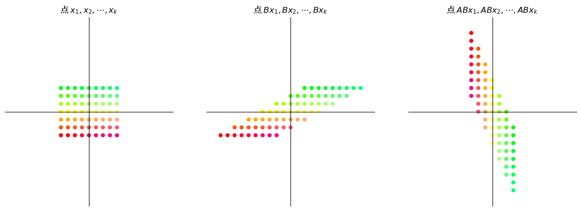
_images/ec445ce1349af7b50405fb0bbcc8785935991ce743e0d16c347c4bb5f87a348e.png

16.4.2.2. 旋转后剪切#

grid_composition_transform(B, A)         # 变换 BA

_images/2d2c7f797bf6087381350f8892777ffd412525ac66737721402062f371b4354f.png

很显然，变换 $A B$ 与变换 $B A$ 是不同的。

16.5. 对固定映射进行迭代#

在经济学（尤其是动态建模）中，我们经常对重复应用固定矩阵所产生的变换感兴趣。

例如，给定一个向量 $v$ 和一个矩阵 $A$ ，我们希望可以研究以下序列：

v, A v, A A v = A^{2} v, \dots

让我们首先看一下在不同映射 $A$ 下的迭代序列 $(A^{k} v)_{k \geq 0}$ 的例子。

def plot_series(A, v, n):

    B = np.array([[1, -1],
                  [1, 0]])

    fig, ax = plt.subplots()

    ax.set(xlim=(-4, 4), ylim=(-4, 4))
    ax.set_xticks([])
    ax.set_yticks([])
    for spine in ['left', 'bottom']:
        ax.spines[spine].set_position('zero')
    for spine in ['right', 'top']:
        ax.spines[spine].set_color('none')

    θ = np.linspace(0, 2 * np.pi, 150)
    r = 2.5
    x = r * np.cos(θ)
    y = r * np.sin(θ)
    x1 = x.reshape(1, -1)
    y1 = y.reshape(1, -1)
    xy = np.concatenate((x1, y1), axis=0)

    ellipse = B @ xy
    ax.plot(ellipse[0, :], ellipse[1, :], color='black',
            linestyle=(0, (5, 10)), linewidth=0.5)

    #初始化轨迹容器
    colors = plt.cm.rainbow(np.linspace(0, 1, 20))

    for i in range(n):
        iteration = matrix_power(A, i) @ v
        v1 = iteration[0]
        v2 = iteration[1]
        ax.scatter(v1, v2, color=colors[i])
        if i == 0:
            ax.text(v1+0.25, v2, f'$v$')
        elif i == 1:
            ax.text(v1+0.25, v2, f'$Av$')
        elif 1 < i < 4:
            ax.text(v1+0.25, v2, f'$A^{i}v$')
    plt.show()

A = np.array([[sqrt(3) + 1, -2],
              [1, sqrt(3) - 1]])
A = (1/(2*sqrt(2))) * A
v = (-3, -3)
n = 12

plot_series(A, v, n)

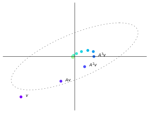
_images/9ced777f16d19e89fb2bc2aaa592659dc2d2fb14b60505c9f381706515c0eb8e.png

每次迭代后，向量变得更短，即更靠近原点。

在这种情况下，重复将向量乘以 $A$ 会使向量”螺旋式地向内”。

B = np.array([[sqrt(3) + 1, -2],
              [1, sqrt(3) - 1]])
B = (1/2) * B
v = (2.5, 0)
n = 12

plot_series(B, v, n)

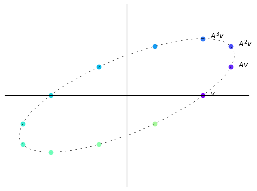
_images/b972eb0c72f8cd89ea3c6a033b580b58756f65903acbb44d6f8cbe20567d186c.png

在这里，每次迭代向量不会变长或变短。

在这种情况下，重复将向量乘以 $A$ 只会使其”围绕一个椭圆旋转”。

B = np.array([[sqrt(3) + 1, -2],
              [1, sqrt(3) - 1]])
B = (1/sqrt(2)) * B
v = (-1, -0.25)
n = 6

plot_series(B, v, n)

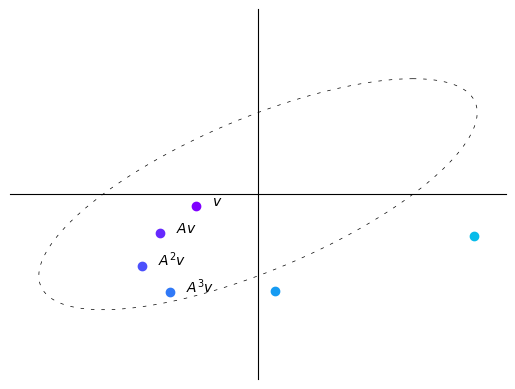
_images/122313210dbad73aa3c02ac616d43c0a96407a0f275e99c4b9fca65bc5ec7009.png

在这里，每次迭代向量趋向于变长，即离原点更远。

在这种情况下，重复将向量乘以 $A$ 会使向量”螺旋式地向外”。

因此，我们观察到序列 $(A^{k} v)_{k \geq 0}$ 的行为取决于映射 $A$ 本身。

现在我们讨论决定这种行为的 $A$ 的性质。

16.6. 特征值#

在本节中，我们引入特征值和特征向量的概念。

16.6.1. 定义#

设 $A$ 为 $n \times n$ 的方阵。

如果存在标量 $λ$ 和非零 $n$ 维向量 $v$ ，使得

A v = λ v .

则我们称 $λ$ 为 $A$ 的 特征值 ， $v$ 为相应的 特征向量。

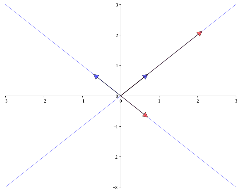
因此， $A$ 的特征向量是一个非零向量 $v$ ，当映射 $A$ 应用于它时， $v$ 仅仅是被缩放。

下图显示了两个特征向量（蓝色箭头）及其在 $A$ 下的像（红色箭头）。

如预期的那样，每个 $v$ 的像 $A v$ 只是原始向量的缩放。

from numpy.linalg import eig

A = [[1, 2],
     [2, 1]]
A = np.array(A)
evals, evecs = eig(A)
evecs = evecs[:, 0], evecs[:, 1]

fig, ax = plt.subplots(figsize=(10, 8))
# 将坐标轴设置为通过原点
for spine in ['left', 'bottom']:
    ax.spines[spine].set_position('zero')
for spine in ['right', 'top']:
    ax.spines[spine].set_color('none')
# ax.grid(alpha=0.4)

xmin, xmax = -3, 3
ymin, ymax = -3, 3
ax.set(xlim=(xmin, xmax), ylim=(ymin, ymax))

# 绘制每个特征向量
for v in evecs:
    ax.annotate('', xy=v, xytext=(0, 0),
                arrowprops=dict(facecolor='blue',
                shrink=0,
                alpha=0.6,
                width=0.5))

# 绘制每个特征向量
for v in evecs:
    v = A @ v
    ax.annotate('', xy=v, xytext=(0, 0),
                arrowprops=dict(facecolor='red',
                shrink=0,
                alpha=0.6,
                width=0.5))

# 绘制它们经过的直线
x = np.linspace(xmin, xmax, 3)
for v in evecs:
    a = v[1] / v[0]
    ax.plot(x, a * x, 'b-', lw=0.4)

plt.show()

_images/0c2f6de6967917fdafde51b5d94f44feea482702d808141930dd05692b458f4e.png

16.6.2. 复数值#

到目前为止，我们对特征值和特征向量的定义似乎很直观。

但还有一个我们尚未提到的复杂情况：

在求解 $A v = λ v$ 时，

$λ$ 可以是复数，并且
$v$ 可以是一个包含 n 个复数的向量。

我们将在下面看到一些例子。

16.6.3. 一些数学细节#

我们为有兴趣的读者注明一些数学细节。（其他读者可以跳到下一节。）

特征值方程等价于 $(A - λ I) v = 0$ 。

只有当 $A - λ I$ 的列线性相关时，这个方程才有非零解 $v$ 。

这反过来等价于行列式为零。

因此，要找到所有特征值，我们可以寻找使 $A - λ I$ 的行列式为零的 $λ$ 。

这个问题可以表示为求解一个 $λ$ 的 n 次多项式的根。

这进而意味着在复平面上存在 n 个解，尽管有些可能是重复的。

16.6.4. 事实#

关于方阵 $A$ 的特征值，有一些很好的事实：

$A$ 的行列式等于其特征值的乘积
$A$ 的迹（主对角线上元素的和）等于其特征值的和
如果 $A$ 是对称的，那么它的所有特征值都是实数
如果 $A$ 可逆，且 $λ_{1}, \dots, λ_{n}$ 是它的特征值，那么 $A^{- 1}$ 的特征值是 $1 / λ_{1}, \dots, 1 / λ_{n}$ 。

最后一个陈述的一个推论是，当且仅当矩阵的所有特征值都非零时，该矩阵才是可逆的。

16.6.5. 计算#

使用 NumPy，我们可以按如下方式求解矩阵的特征值和特征向量

from numpy.linalg import eig

A = ((1, 2),
     (2, 1))

A = np.array(A)
evals, evecs = eig(A)
evals  # 特征值

array([ 3., -1.])

evecs  # 特征向量

array([[ 0.70710678, -0.70710678],
       [ 0.70710678,  0.70710678]])

请注意，evecs 的列是特征向量。

由于特征向量的任何标量倍数都是具有相同特征值的特征向量（可以试着验证一下），eig 程序将每个特征向量的长度归一化为1。

映射 $A$ 的特征向量和特征值决定了当我们反复乘以 $A$ 时，向量 $v$ 如何被变换。

这一点将在后面进一步讨论。

16.7. 诺伊曼级数引理#

在本节中，我们将介绍一个关于矩阵级数的著名结果，它在经济学中有许多应用。

16.7.1. 标量级数#

以下是关于级数的一个基本结果：

如果 $a$ 是一个数，且 $| a | < 1$ ，那么

(16.1)#

\sum_{k = 0}^{\infty} a^{k} = \frac{1}{1 - a} = (1 - a)^{- 1}

对于一维线性方程 $x = a x + b$ ，其中 x 未知，我们可以得出解 $x^{*}$ 由以下给出：

x^{*} = \frac{b}{1 - a} = \sum_{k = 0}^{\infty} a^{k} b

16.7.2. 矩阵级数#

这个想法在矩阵设置中也有一个推广。

考虑方程组 $x = A x + b$ ，其中 $A$ 是一个 $n \times n$ 的方阵， $x$ 和 $b$ 都是 $R^{n}$ 中的列向量。

使用矩阵代数，我们可以得出这个方程组的解由以下给出：

(16.2)#

x^{*} = (I - A)^{- 1} b

什么条件保证了存在唯一的向量 $x^{*}$ 满足方程 (16.2)？

以下是泛函分析中的一个基本结果，它将 (16.1) 推广到多变量情况。

Theorem 16.1 (诺伊曼级数引理)

设 $A$ 为方阵， $A^{k}$ 为 $A$ 的 $k$ 次幂。设 $r (A)$ 为 $A$ 的谱半径，定义为 $max_{i} | λ_{i} |$ ，其中

${λ_{i}}_{i}$ 是 $A$ 的特征值集，且
$| λ_{i} |$ 是复数 $λ_{i}$ 的模

诺伊曼定理陈述如下：如果 $r (A) < 1$ ，那么 $I - A$ 是可逆的，且

(I - A)^{- 1} = \sum_{k = 0}^{\infty} A^{k}

我们可以在以下例子中看到诺伊曼级数引理的应用。

A = np.array([[0.4, 0.1],
              [0.7, 0.2]])

evals, evecs = eig(A)   #求出特征值和特征向量

r = max(abs(λ) for λ in evals)    # 计算谱半径
print(r)

0.5828427124746189

获得的谱半径 $r (A)$ 小于1。

因此，我们可以应用诺伊曼级数引理来求 $(I - A)^{- 1}$ 。

I = np.identity(2)  # 2 x 2 单位矩阵
B = I - A

B_inverse = np.linalg.inv(B)  # 直接求逆

A_sum = np.zeros((2, 2))  # A 的幂级数和
A_power = I
for i in range(50):
    A_sum += A_power
    A_power = A_power @ A

让我们检查求和方法和逆序方法的结果是否相等。

np.allclose(A_sum, B_inverse)

True

虽然我们在 $k = 50$ 时截断了无限级数，但两种方法给出了相同的结果，这体现了诺伊曼级数引理的结论。

16.8. 练习#

Exercise 16.1

幂迭代法是一种用于寻找可对角化矩阵最大绝对特征值的方法。

该方法从一个随机向量 $b_{0}$ 开始，重复地对其应用矩阵 $A$

b_{k + 1} = \frac{A b_{k}}{‖ A b_{k} ‖}

关于该方法的详细讨论可以在这里找到。

在这个练习中，首先实现幂迭代方法，并用它来找出最大绝对特征值及其对应的特征向量。

然后可视化收敛过程。

Solution to Exercise 16.1

这里有一个解决方案。

我们首先研究特征向量近似值与真实特征向量之间的距离。

# 定义矩阵A
A = np.array([[1, 0, 3],
              [0, 2, 0],
              [3, 0, 1]])

num_iters = 20

# 定义一个随机的初始向量 b
b = np.random.rand(A.shape[1])

# 获取矩阵A的主特征向量
eigenvector = np.linalg.eig(A)[1][:, 0]

errors = []
res = []

# 幂迭代循环
for i in range(num_iters):
    # Multiply b by A
    b = A @ b
    # 归一化b
    b = b / np.linalg.norm(b)
    # 将b添加到特征向量近似值列表中
    res.append(b)
    err = np.linalg.norm(np.array(b)
                         - eigenvector)
    errors.append(err)

greatest_eigenvalue = np.dot(A @ b, b) / np.dot(b, b)
print(f'近似的最大绝对特征值是 \
        {greatest_eigenvalue:.2f}')
print('真实的特征值是', np.linalg.eig(A)[0])

# 绘制每次迭代的特征向量近似值
plt.figure(figsize=(10, 6))
plt.xlabel('次数')
plt.ylabel('误差')
_ = plt.plot(errors)

近似的最大绝对特征值是         4.00
真实的特征值是 [ 4. -2.  2.]

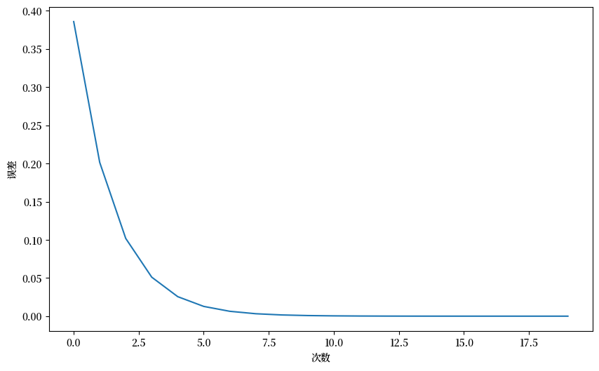
_images/fe38ca6378c242469bfca7419f09008bd15d1b24cff364ed857eb0a22e4c0127.png — Fig. 16.1 Power iteration#

然后我们可以观察特征向量近似值的轨迹。

# 设置3D图形和坐标轴
fig = plt.figure()
ax = fig.add_subplot(111, projection='3d')

# 绘制特征向量
ax.scatter(eigenvector[0],
           eigenvector[1],
           eigenvector[2],
           color='r', s=80)

for i, vec in enumerate(res):
    ax.scatter(vec[0], vec[1], vec[2],
               color='b',
               alpha=(i+1)/(num_iters+1),
               s=80)

ax.set_xlabel('x')
ax.set_ylabel('y')
ax.set_zlabel('z')
ax.tick_params(axis='both', which='major', labelsize=7)

points = [plt.Line2D([0], [0], linestyle='none',
                     c=i, marker='o') for i in ['r', 'b']]
ax.legend(points, ['真正的特征向量',
                   r'近似的特征向量 ($b_k$)'])
ax.set_box_aspect(aspect=None, zoom=0.8)

plt.show()

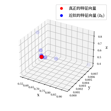
_images/258196f1b1ebd9ff2c834516762e9eb32e320cb8d9f297133c943b925c51ee6c.png — Fig. 16.2 Power iteration trajectory#

Exercise 16.2

我们已经讨论了向量 $v$ 经过矩阵 $A$ 变换后的轨迹。

考虑矩阵 $A = [\begin{matrix} 1 & 2 \\ 1 & 1 \end{matrix}]$ 和向量 $v = [\begin{matrix} 2 \\ - 2 \end{matrix}]$ 。

尝试计算向量 $v$ 经过矩阵 $A$ 变换 $n = 4$ 次迭代后的轨迹，并绘制结果。

Solution to Exercise 16.2

A = np.array([[1, 2],
              [1, 1]])
v = (0.4, -0.4)
n = 11

# 计算特征值和特征向量
eigenvalues, eigenvectors = np.linalg.eig(A)

print(f'特征值:\n {eigenvalues}')
print(f'特征向量:\n {eigenvectors}')

plot_series(A, v, n)

特征值:
 [ 2.41421356 -0.41421356]
特征向量:
 [[ 0.81649658 -0.81649658]
 [ 0.57735027  0.57735027]]

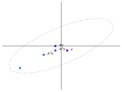
_images/1fe5955a14d4268e0613aba9fa5ca5d05a4bd97233937d0e449b24479f5d8bcc.png

结果似乎收敛于矩阵 $A$ 最大特征值对应的特征向量。

让我们使用向量场来可视化矩阵 $A$ 带来的变换。（这是线性代数中的一个较高级话题，如果你对数学感到足够自信和感兴趣的话，可以继续往下学习。）

# 创建格点
x, y = np.meshgrid(np.linspace(-5, 5, 15),
                   np.linspace(-5, 5, 20))

#将矩阵A应用于向量场中的每个点
vec_field = np.stack([x, y])
u, v = np.tensordot(A, vec_field, axes=1)

# 绘制转换后的向量场
c = plt.streamplot(x, y, u - x, v - y,
                   density=1, linewidth=None, color='#A23BEC')
c.lines.set_alpha(0.5)
c.arrows.set_alpha(0.5)

# 绘制特征向量
origin = np.zeros((2, len(eigenvectors)))
parameters = {'color': ['b', 'g'], 'angles': 'xy',
              'scale_units': 'xy', 'scale': 0.1, 'width': 0.01}
plt.quiver(*origin, eigenvectors[0],
           eigenvectors[1], **parameters)
plt.quiver(*origin, - eigenvectors[0],
           - eigenvectors[1], **parameters)

colors = ['b', 'g']
lines = [Line2D([0], [0], color=c, linewidth=3) for c in colors]
labels = ["2.4 特征空间", "0.4 特征空间"]
plt.legend(lines, labels, loc='center left',
           bbox_to_anchor=(1, 0.5))

plt.xlabel("x")
plt.ylabel("y")
plt.grid()
plt.gca().set_aspect('equal', adjustable='box')
plt.show()

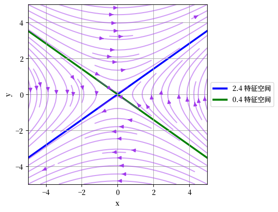
_images/b58181228e736592fad5c86f73486f4d27a049169fd2b5f06763c939390e9779.png — Fig. 16.3 收敛于特征向量#

请注意，向量场收敛于 $A$ 的最大特征值对应的特征向量，并从 $A$ 的最小特征值对应的特征向量发散。

实际上，特征向量也是矩阵 $A$ 拉伸或压缩空间的方向。

具体来说，最大特征值对应的特征向量是矩阵 $A$ 最大程度拉伸空间的方向。

我们将在接下来的练习中看到更多有趣的例子。

Exercise 16.3

之前，我们展示了向量 $v$ 被三种不同矩阵 $A$ 变换后的轨迹。

使用前面练习中的可视化来解释向量 $v$ 被这三种不同矩阵 $A$ 变换后的轨迹。

Solution to Exercise 16.3

以下是其中一种解法。

figure, ax = plt.subplots(1, 3, figsize=(15, 5))
A = np.array([[sqrt(3) + 1, -2],
              [1, sqrt(3) - 1]])
A = (1/(2*sqrt(2))) * A

B = np.array([[sqrt(3) + 1, -2],
              [1, sqrt(3) - 1]])
B = (1/2) * B

C = np.array([[sqrt(3) + 1, -2],
              [1, sqrt(3) - 1]])
C = (1/sqrt(2)) * C

examples = [A, B, C]

for i, example in enumerate(examples):
    M = example

    # 计算特征向量和特征值
    eigenvalues, eigenvectors = np.linalg.eig(M)
    print(f'实例 {i+1}:\n')
    print(f'特征值:\n {eigenvalues}')
    print(f'特征向量:\n {eigenvectors}\n')

    eigenvalues_real = eigenvalues.real
    eigenvectors_real = eigenvectors.real

    # 创建格点
    x, y = np.meshgrid(np.linspace(-20, 20, 15),
                       np.linspace(-20, 20, 20))

    # 将矩阵A应用于向量场中的每个点
    vec_field = np.stack([x, y])
    u, v = np.tensordot(M, vec_field, axes=1)

    # 绘制转换后的向量场
    c = ax[i].streamplot(x, y, u - x, v - y, density=1,
                         linewidth=None, color='#A23BEC')
    c.lines.set_alpha(0.5)
    c.arrows.set_alpha(0.5)

    # 绘制特征向量
    parameters = {'color': ['b', 'g'], 'angles': 'xy',
                  'scale_units': 'xy', 'scale': 1,
                  'width': 0.01, 'alpha': 0.5}
    origin = np.zeros((2, len(eigenvectors)))
    ax[i].quiver(*origin, eigenvectors_real[0],
                 eigenvectors_real[1], **parameters)
    ax[i].quiver(*origin,
                 - eigenvectors_real[0],
                 - eigenvectors_real[1],
                 **parameters)

    ax[i].set_xlabel("x-axis")
    ax[i].set_ylabel("y-axis")
    ax[i].grid()
    ax[i].set_aspect('equal', adjustable='box')

plt.show()

实例 1:

特征值:
 [0.61237244+0.35355339j 0.61237244-0.35355339j]
特征向量:
 [[0.81649658+0.j         0.81649658-0.j        ]
 [0.40824829-0.40824829j 0.40824829+0.40824829j]]

实例 2:

特征值:
 [0.8660254+0.5j 0.8660254-0.5j]
特征向量:
 [[0.81649658+0.j         0.81649658-0.j        ]
 [0.40824829-0.40824829j 0.40824829+0.40824829j]]

实例 3:

特征值:
 [1.22474487+0.70710678j 1.22474487-0.70710678j]
特征向量:
 [[0.81649658+0.j         0.81649658-0.j        ]
 [0.40824829-0.40824829j 0.40824829+0.40824829j]]

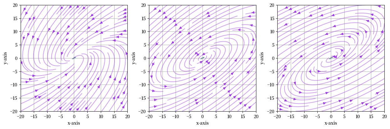
_images/14cf33627e3a1492c2266fef21ab97569ce10a92c5af8a35ece8423e2360b27e.png — Fig. 16.4 三个不同矩阵的向量场#

这些向量场解释了为什么我们之前观察到向量 $v$ 被矩阵 $A$ 反复相乘后的轨迹。

这里展示的模式是因为我们有复数特征值和特征向量。

我们可以使用从stackoverflow获取的Arrow3D类来为其中一个矩阵绘制复平面。

class Arrow3D(FancyArrowPatch):
    def __init__(self, xs, ys, zs, *args, **kwargs):
        super().__init__((0, 0), (0, 0), *args, **kwargs)
        self._verts3d = xs, ys, zs

    def do_3d_projection(self):
        xs3d, ys3d, zs3d = self._verts3d
        xs, ys, zs = proj3d.proj_transform(xs3d, ys3d, zs3d,
                                           self.axes.M)
        self.set_positions((0.1*xs[0], 0.1*ys[0]),
                           (0.1*xs[1], 0.1*ys[1]))

        return np.min(zs)


eigenvalues, eigenvectors = np.linalg.eig(A)

#为向量场创建网格
x, y = np.meshgrid(np.linspace(-2, 2, 15),
                   np.linspace(-2, 2, 15))

# 计算向量场（实部和虚部）
u_real = A[0][0] * x + A[0][1] * y
v_real = A[1][0] * x + A[1][1] * y
u_imag = np.zeros_like(x)
v_imag = np.zeros_like(y)

# 创建3D图像
fig = plt.figure()
ax = fig.add_subplot(111, projection='3d')
vlength = np.linalg.norm(eigenvectors)
ax.quiver(x, y, u_imag, u_real-x, v_real-y, v_imag-u_imag,
          colors='b', alpha=0.3, length=.2,
          arrow_length_ratio=0.01)

arrow_prop_dict = dict(mutation_scale=5,
                       arrowstyle='-|>', shrinkA=0, shrinkB=0)

# 绘制3D特征向量
for c, i in zip(['b', 'g'], [0, 1]):
    a = Arrow3D([0, eigenvectors[0][i].real],
                [0, eigenvectors[1][i].real],
                [0, eigenvectors[1][i].imag],
                color=c, **arrow_prop_dict)
    ax.add_artist(a)

# 设置坐标轴标签和标题
ax.set_xlabel('x')
ax.set_ylabel('y')
ax.set_zlabel('Im')
ax.set_box_aspect(aspect=None, zoom=0.8)

plt.draw()
plt.show()

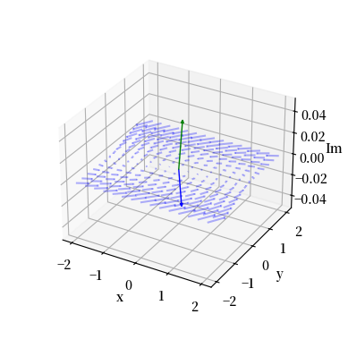
_images/eaf2978ade88496e9a4cce150503e7da3cd7033524259e23615a3699bc46432d.png — Fig. 16.5 向量场的三维图（复平面）#