4. 通货膨胀的历史#
本讲将透过一些历史数据探讨价格指数的波动模式及其背后的故事。
首先,我们需要安装一些必要的Python包。
注意:我们安装xlrd是因为pandas在读取Excel文件时需要它。
!pip install xlrd
我们现在导入本讲所需的Python库。
import numpy as np
import pandas as pd
import matplotlib.pyplot as plt
import matplotlib.dates as mdates

import matplotlib as mpl
FONTPATH = "fonts/SourceHanSerifSC-SemiBold.otf"
mpl.font_manager.fontManager.addfont(FONTPATH)
plt.rcParams['font.family'] = ['Source Han Serif SC']
价格水平的增长率在媒体和央行及财政官员的口中被称为通货膨胀。
价格水平衡量的是一篮子消费品在国内货币单位中的价值。
例如,在美国,\(t\)时期的价格水平表示购买一单位标准消费品篮子所需的美元数量(以\(t\)月或\(t\)年计)。
在20世纪之前,许多西方经济体的价格水平虽然存在短期波动,但长期来看并没有明显的上升或下降趋势。
一个世纪开始时的价格水平通常与该世纪结束时的水平相差不大。
然而,20世纪的情况发生了显著变化,这一点我们将在本讲中详细探讨。
这种变化的一个普遍接受的解释是,20世纪初期各国逐渐放弃了以黄金和白银作为货币基础的金本位和银本位制度。
Tip
本讲为后续几讲做好了铺垫,这些后续几讲中我们将用宏观经济学家的角度来思考决定价格水平的因素,即货币主义价格水平理论 和 自适应预期下的货币主义价格水平理论
4.1. 四个世纪的价格水平#
我们首先展示最初出现在 [Sargent and Velde, 2002] 第35页的数据,其中包含了自1600年到1914年四个“硬通货”国家的价格水平。
法国
西班牙(卡斯蒂利亚)
英国
美国
在当前语境中,“硬通货”一词意味着这些国家采用了商品货币标准:货币由金银币组成,这些金银币的流通价值主要由它们的金银含量决定。
Note
在金本位或银本位制下,一些货币还包括”仓单”,即代表对金币或银币索赔权的纸质凭证。政府或私人银行发行的钞票可以被视为这种”仓单”的例子。
我们用 pandas导入一个数据集。
# 导入数据并清理索引
data_url = "https://github.com/QuantEcon/lecture-python-intro/raw/main/lectures/datasets/longprices.xls"
df_fig5 = pd.read_excel(data_url,
                        sheet_name='all',
                        header=2,
                        index_col=0).iloc[1:]
df_fig5.index = df_fig5.index.astype(int)
我们首先绘制1600年至1914年间的价格水平。
在这段时间的大多数年份内,这些国家采用金本位或银本位。
df_fig5_befe1914 = df_fig5[df_fig5.index <= 1914]

# 创建图表
cols = ['UK', 'US', 'France', 'Castile']
cols_cn = ['英国', '美国', '法国', '卡斯蒂利亚(西班牙)']

fig, ax = plt.subplots(figsize=(10,6))

for col, col_cn in zip(cols, cols_cn):
    ax.plot(df_fig5_befe1914.index,
            df_fig5_befe1914[col], label=col_cn, lw=2)

ax.legend()
ax.set_ylabel('指数 1913 = 100')
ax.set_xlabel('年份')
ax.set_xlim(xmin=1600)
plt.tight_layout()
plt.show()
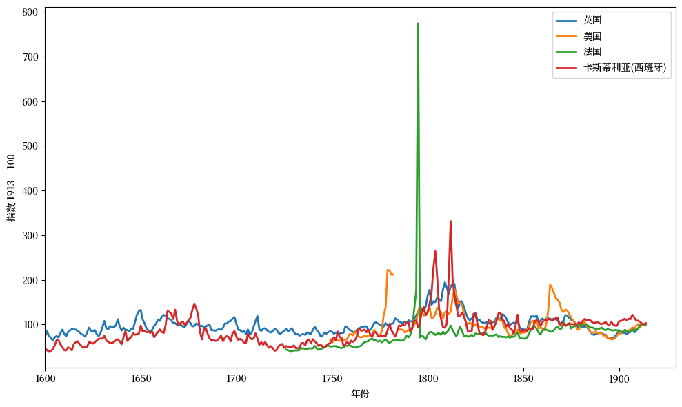
Fig. 4.1 长期价格水平时间序列#
我们说“大多数年份”是因为金本位或银本位制度曾经有过暂时的中断。
通过仔细观察 Fig. 4.1,你可能能猜到这些中断发生的时间,因为这些时期的价格水平出现了显著的暂时性上涨:
1791-1797年的法国(法国大革命)
1776-1790年的美国(从大英帝国独立的战争)
1861-1865年的美国(南北战争)
在这些事件期间,当政府为了支付战争支出而印制纸币时,金银本位被暂时放弃。
Note
法国大革命期间的通货膨胀 讲述了在法国大革命期间发生的大通胀的历史。
尽管出现了这些暂时的中断,图中一个显著的特点是三个世纪以来价格水平大致保持恒定。
在这个世纪初期,这些数据的另外两个特点引起了耶鲁大学的欧文·费雪(Irving Fisher)和剑桥大学的约翰·梅纳德·凯恩斯(John Maynard Keynes)的关注。
尽管长期锚定在相同的平均水平上,年度价格水平的波动还是很大
虽然使用有价值的黄金和白银作为货币成功地通过限制货币供给稳定了价格水平,但这需要消耗现实的资源 –
一个国家使用金银币作为货币支付了高昂的“机会成本”——那些金银本可以制成有价值的珠宝和其他耐用品。
凯恩斯和费雪提出了他们认为可以更有效地实现价格水平稳定的方式:
既能像金银本位下一样稳固地锚定价格水平,
也能减少年度短期波动。
他们说,中央银行可以通过以下方式实现价格水平的稳定
发行有限供应的纸币
拒绝印制钞票为政府支出提供资金
这种逻辑促使约翰·梅纳德·凯恩斯称商品本位制为 “野蛮的遗物”。
纸币或 “法定货币 ”体系使货币脱离其背后支持它的储备。
但是,坚持金本位制或银本位制提供了一种自动限制货币供应量的机制,从而锚定了价格水平。
为了锚定价格水平,纯粹的纸币或法定货币体系用中央银行取代了这一自动机制,中央银行拥有限制货币供应的权力和决心(并能阻止造假者!)。
现在,让我们通过展示原载于[Sargent and Velde, 2002]第35页的完整图表,来看看1914年之后,当四个国家相继脱离金/银本位制时,它们的物价水平发生了什么变化。
fig, ax = plt.subplots(dpi=200)

for col, col_cn in zip(cols, cols_cn):
    ax.plot(df_fig5.index, df_fig5[col], lw=2)
    ax.text(x=df_fig5.index[-1]+2,
            y=df_fig5[col].iloc[-1], s=col_cn)

ax.set_yscale('log')
ax.set_ylabel('价格水平对数(指数1913=100)')
ax.set_ylim([10, 1e6])
ax.set_xlabel('年份')
ax.set_xlim(xmin=1600)
plt.tight_layout()
plt.show()
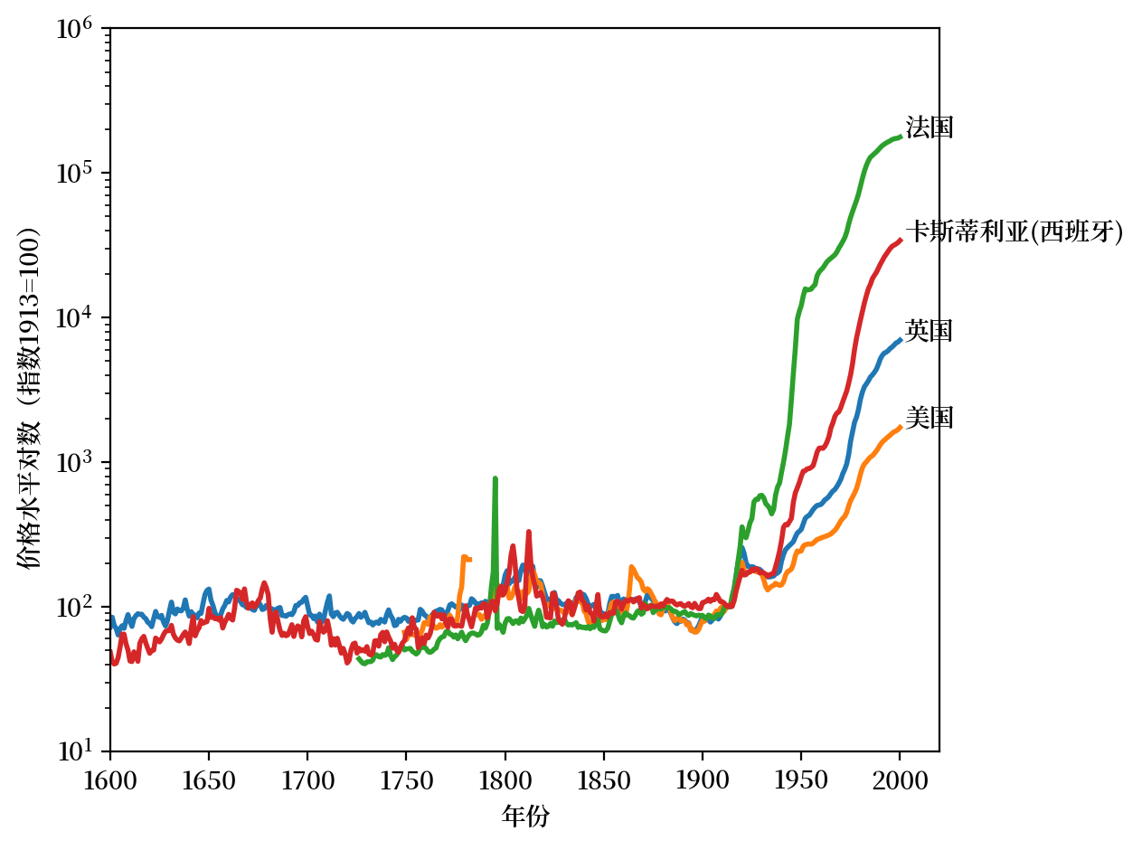
Fig. 4.2 长期价格水平时间序列(对数)#
Fig. 4.2显示,印制纸币的中央银行在锚定价格水平方面的表现不如金本位和银本位。
这可能会让凯恩斯和费雪感到惊讶或失望。
事实上,早在凯恩斯和费雪在20世纪初倡导法定货币制度之前,早期的经济学家和政治家们就知道法定货币制度的可能性。
商品货币体系的支持者不相信政府和中央银行能够妥善管理法定货币体系。
他们愿意支付与建立和维护商品货币体系相关的资源成本。
鉴于许多国家在20世纪放弃商品货币后经历了持续的高通胀,我们也可以理解为什么金本位制或银本位制的倡导者倾向于维持1914年前的金/银本位制。
二十世纪在纸币法定本位制下经历的通货膨胀的广度和长度在历史上都是前所未有的。
4.2. 四次大通胀#
在 1918 年 11 月结束的第一次世界大战之后,货币和财政当局艰难地在尝试不实行金本位或银本位的情况下实现价格水平的稳定。
我们展示了[Sargent, 2013]第3章 “四次大通胀的结局” 中的四幅图。
这些图表描述了第一次世界大战后初期四个国家价格水平的对数:
图 3.1:1921-1924 年奥地利的零售价格(第 42 页)
图 3.2:1921-1924 年匈牙利的批发价格(第 43 页)
图 3.3:批发价格,波兰,1921-1924 年(第 44 页)
图 3.4:批发价格,德国,1919-1924 年(第 45 页)
我们在四幅图中的每一幅都加上了相对美元汇率的对数。
图表的基础数据载于[Sargent, 2013]第3章附录中的表格。
我们将所有这些数据转录到电子表格 chapter_3.xlsx 中,并将其读入 pandas。
在下面的代码单元中,我们将清理数据并构建一个 pandas.dataframe。
现在,我们编写绘图函数 pe_plot 和 pr_plot ,它们将绘制出价格水平、汇率、和通货膨胀率的图表。
接下来我们为每个国家准备数据
# 导入数据
data_url = "https://github.com/QuantEcon/lecture-python-intro/raw/main/lectures/datasets/chapter_3.xlsx"
xls = pd.ExcelFile(data_url)

# 选择相关的数据表
sheet_index = [(2, 3, 4),
               (9, 10),
               (14, 15, 16),
               (21, 18, 19)]

# 删除多余的行
remove_row = [(-2, -2, -2),
              (-7, -10),
              (-6, -4, -3),
              (-19, -3, -6)]

# 对每个国家的序列进行解包和合并
df_list = []

for i in range(4):

    indices, rows = sheet_index[i], remove_row[i]

    # 在选定的工作表上应用 process_entry
    sheet_list = [
        pd.read_excel(xls, 'Table3.' + str(ind),
            header=1).iloc[:row].map(process_entry)
        for ind, row in zip(indices, rows)]

    sheet_list = [process_df(df) for df in sheet_list]
    df_list.append(pd.concat(sheet_list, axis=1))

df_aus, df_hun, df_pol, df_deu = df_list
现在,我们为四个国家绘制图表。
我们将为每个国家绘制两幅图。
第一幅图绘制的是
价格水平
相对于美元的汇率
对于每个国家,图表右侧的刻度与价格水平相关,而图表左侧的刻度与汇率相关。
对于每个国家,第二张图表绘制的是通货膨胀率的三个月居中移动平均值,定义为 \(\frac{p_{t-1}+p_t+p_{t+1}}{3}\)。
4.2.1. 奥地利#
我们的数据来源是
表 3.3,零售价格水平 \(\exp p\)
表 3.4,与美国的汇率
p_seq = df_aus['Retail price index, 52 commodities']
e_seq = df_aus['Exchange Rate']

lab = ['零售价格指数',
       '奥地利克朗兑美分']

# 创建图表
fig, ax = plt.subplots(dpi=200)
ax1 = pe_plot(p_seq, e_seq, df_aus.index, lab, ax)
ax1.xaxis.set_major_locator(mdates.MonthLocator(interval=8))
ax1.xaxis.set_major_formatter(mdates.DateFormatter('%Y年%m月'))

plt.show()
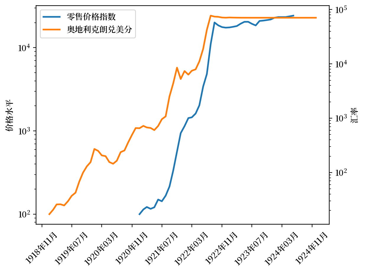
Fig. 4.3 价格指数和汇率(奥地利)#
# 绘制移动平均线
fig, ax = plt.subplots(dpi=200)
ax1 = pr_plot(p_seq, df_aus.index, ax)
ax1.xaxis.set_major_locator(mdates.MonthLocator(interval=8))
ax1.xaxis.set_major_formatter(mdates.DateFormatter('%Y年%m月'))

plt.show()
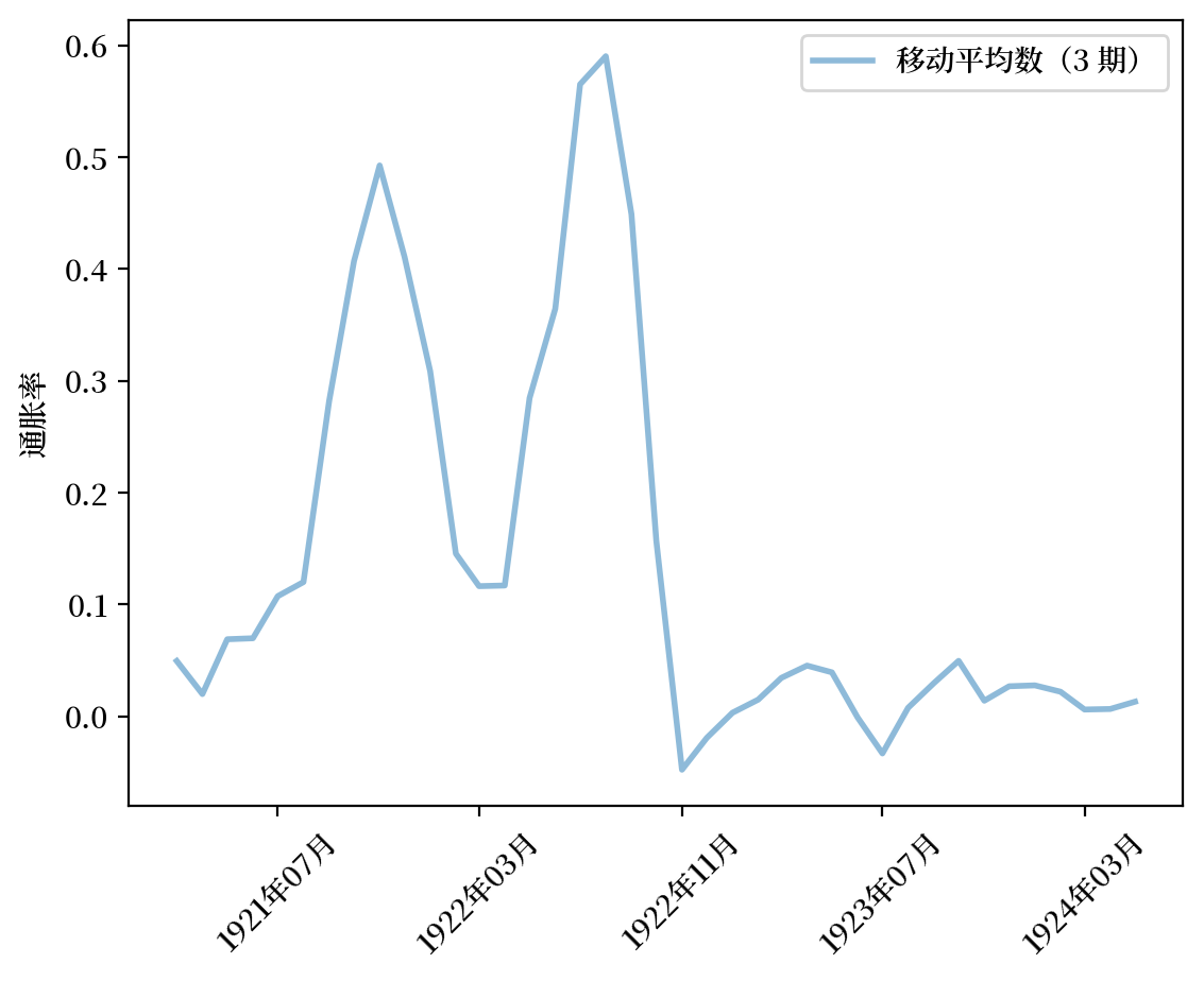
Fig. 4.4 月通货膨胀率(奥地利)#
观察 Fig. 4.3 和 Fig. 4.4 我们可以看到:
“超级通货膨胀”的一段时期中,价格水平的对数迅速上升,月通胀率非常高
超级通货膨胀的突然停止,表现为价格水平的对数的突然变平,以及三个月平均通胀率的显著且永久地下降
美元汇率跟随价格水平走势。
我们将在接下来的三个案例中看到类似的模式。
4.2.2. 匈牙利#
我们的数据来源为:
表 3.10,价格水平 \(\exp p\) 和汇率
p_seq = df_hun['Hungarian index of prices']
e_seq = 1 / df_hun['Cents per crown in New York']

lab = ['匈牙利价格指数',
       '匈牙利克朗兑美分']

# 创建图表
fig, ax = plt.subplots(dpi=200)
ax1 = pe_plot(p_seq, e_seq, df_hun.index, lab, ax)
ax1.xaxis.set_major_locator(mdates.MonthLocator(interval=8))
ax1.xaxis.set_major_formatter(mdates.DateFormatter('%Y年%m月'))

plt.show()
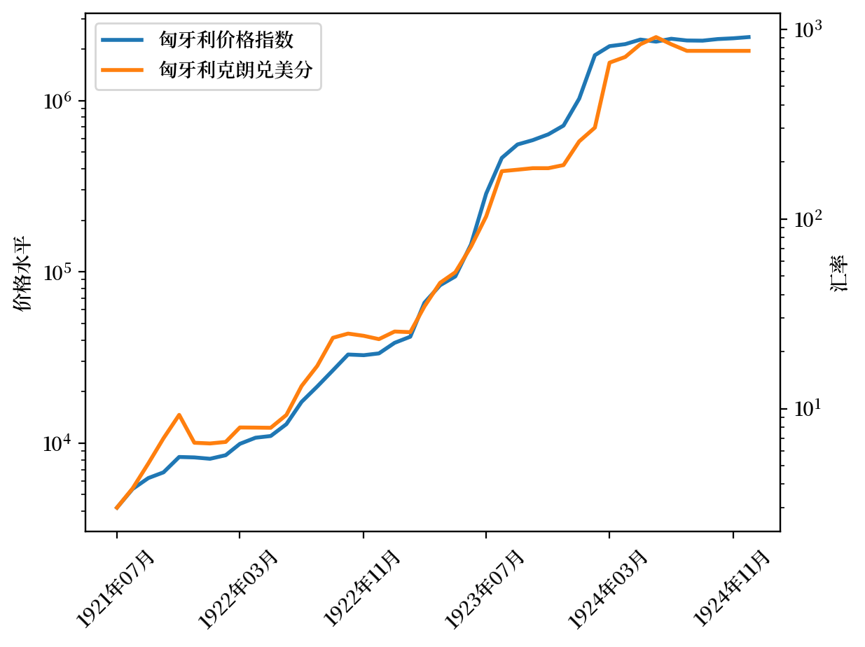
Fig. 4.5 价格指数和汇率(匈牙利)#
# 绘制移动平均线
fig, ax = plt.subplots(dpi=200)
ax1 = pr_plot(p_seq, df_hun.index, ax)
ax1.xaxis.set_major_locator(mdates.MonthLocator(interval=8))
ax1.xaxis.set_major_formatter(mdates.DateFormatter('%Y年%m月'))
plt.show()
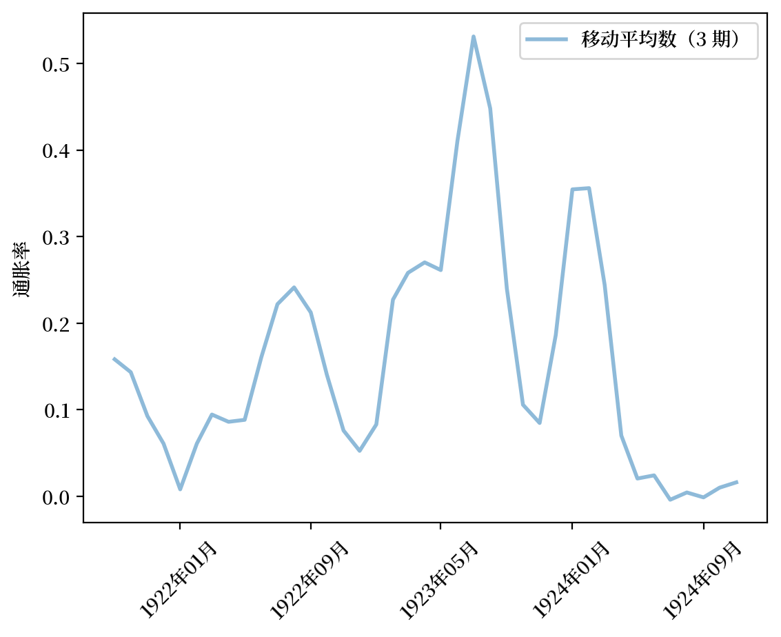
Fig. 4.6 月通货膨胀率(匈牙利)#
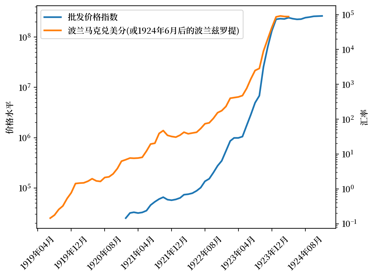
4.2.3. 波兰#
波兰的数据来源如下
表 3.15,价格水平 \(\exp p\)
表 3.15,汇率
Note
为了构建波兰的价格水平序列,我们参照 [Sargent, 2013] 第3章的方法处理电子表格数据。
我们需要将三个不同的价格指数序列连接起来:批发价格指数、基于纸币的批发价格指数,以及1924年6月波兰引入新货币兹罗提后的批发价格指数。
为了确保连接后的序列连续性,我们根据相邻序列重叠期间的价格比率进行了调整,从而创建一个完整的价格水平时间序列。
关于汇率数据,我们只使用到1924年5月的数据,因为6月后波兰采用了新货币兹罗提,而我们缺少以兹罗提计价的价格数据。为了保持一致性,我们使用了旧货币(波兰马克)在6月的汇率进行最后的调整。
# 拼接三个不同单位的价格序列
p_seq1 = df_pol['Wholesale price index'].copy()
p_seq2 = df_pol['Wholesale Price Index: '
                'On paper currency basis'].copy()
p_seq3 = df_pol['Wholesale Price Index: '
                'On zloty basis'].copy()

# 非NaN部分
mask_1 = p_seq1[~p_seq1.isna()].index[-1]
mask_2 = p_seq2[~p_seq2.isna()].index[-2]

adj_ratio12 = (p_seq1[mask_1] / p_seq2[mask_1])
adj_ratio23 = (p_seq2[mask_2] / p_seq3[mask_2])

# 拼接三个序列
p_seq = pd.concat([p_seq1[:mask_1],
                   adj_ratio12 * p_seq2[mask_1:mask_2],
                   adj_ratio23 * p_seq3[mask_2:]])
p_seq = p_seq[~p_seq.index.duplicated(keep='first')]

# 汇率
e_seq = 1/df_pol['Cents per Polish mark (zloty after May 1924)']
e_seq[e_seq.index > '05-01-1924'] = np.nan
lab = ['批发价格指数',
       '波兰马克兑美分(或1924年6月后的波兰兹罗提)']

# 创建图表
fig, ax = plt.subplots(dpi=200)
ax1 = pe_plot(p_seq, e_seq, df_pol.index, lab, ax)
ax1.xaxis.set_major_locator(mdates.MonthLocator(interval=8))
ax1.xaxis.set_major_formatter(mdates.DateFormatter('%Y年%m月'))
plt.show()
# 绘制移动平均线
fig, ax = plt.subplots(dpi=200)
ax1 = pr_plot(p_seq, df_pol.index, ax)
ax1.xaxis.set_major_locator(mdates.MonthLocator(interval=8))
ax1.xaxis.set_major_formatter(mdates.DateFormatter('%Y年%m月'))

plt.show()
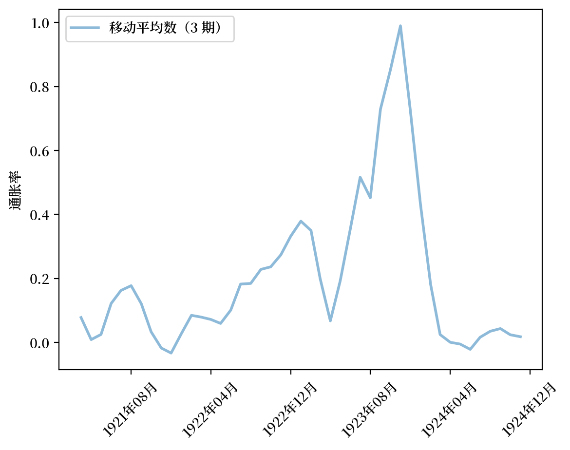
Fig. 4.7 月通货膨胀率(波兰)#
4.2.4. 德国#
德国的数据来源于[Sargent, 2013]第 3 章中的以下表格:
表 3.18,批发价格水平 \(\exp p\)
表 3.19,汇率
p_seq = df_deu['Price index (on basis of marks before July 1924,'
                '  reichsmarks after)'].copy()
e_seq = 1/df_deu['Cents per mark']

lab = ['价格指数',
       '马克兑美分']

# 创建图表
fig, ax = plt.subplots(dpi=200)
ax1 = pe_plot(p_seq, e_seq, df_deu.index, lab, ax)
ax1.xaxis.set_major_locator(mdates.MonthLocator(interval=8))
ax1.xaxis.set_major_formatter(mdates.DateFormatter('%Y年%m月'))

plt.show()
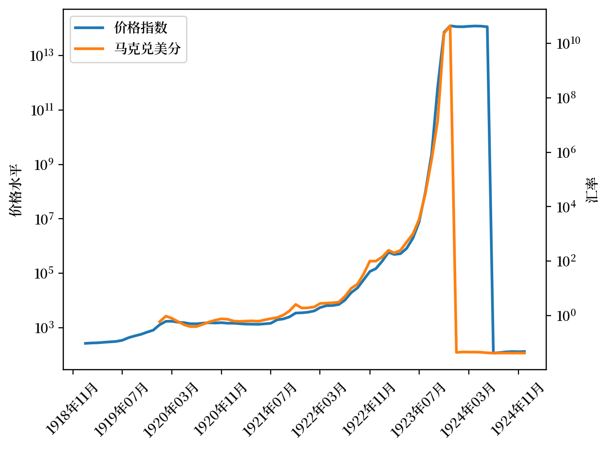
Fig. 4.8 价格指数和汇率(德国)#
p_seq = df_deu['Price index (on basis of marks before July 1924,'
                '  reichsmarks after)'].copy()
e_seq = 1/df_deu['Cents per mark'].copy()

# 货币改革后调整价格水平/汇率
p_seq[p_seq.index > '06-01-1924'] = p_seq[p_seq.index
                                          > '06-01-1924'] * 1e12
e_seq[e_seq.index > '12-01-1923'] = e_seq[e_seq.index
                                          > '12-01-1923'] * 1e12

lab = ['价格指数(马克或换算成马克)',
       '马克兑美分(或德国马克换算成马克)']

# Create plot
fig, ax = plt.subplots(dpi=200)
ax1 = pe_plot(p_seq, e_seq, df_deu.index, lab, ax)
ax1.xaxis.set_major_locator(mdates.MonthLocator(interval=8))
ax1.xaxis.set_major_formatter(mdates.DateFormatter('%Y年%m月'))

plt.show()
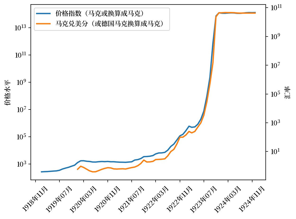
Fig. 4.9 价格指数(调整后)和汇率(德国)#
# 绘制移动平均线
fig, ax = plt.subplots(dpi=200)
ax1 = pr_plot(p_seq, df_deu.index, ax)
ax1.xaxis.set_major_locator(mdates.MonthLocator(interval=8))
ax1.xaxis.set_major_formatter(mdates.DateFormatter('%Y年%m月'))
plt.show()
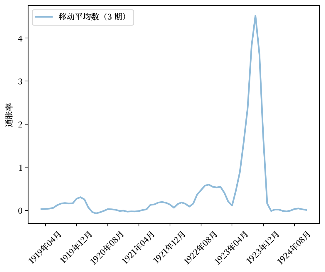
Fig. 4.10 月通胀率(德国)#
4.3. 大通胀的开始和停止#
奥地利、匈牙利、波兰和德国的价格水平在快速上升后,下降得如此之快,这一现象令人瞩目。
这些“突然停止”还表现在上述四个国家的三月移动平均通胀率的永久性下降。
此外,这四个国家的美元汇率走势与其价格水平相似。
Note
这种模式是汇率兑换率理论中购买力平价理论的一个实例。
这些大通胀似乎都“在一瞬间停止”。
[Sargent and Velde, 2002] 的第3章对这一显著模式提供了解释。
简而言之,他们提供的解释如下。
一战后,美国实行了金本位制。
美国政府随时准备按指定数量的金子兑换一美元。
一战后,匈牙利、奥地利、波兰和德国没有立刻实行金本位制。
他们的货币是“法定”或“无支持”的,意思是他们不受政府将其兑换成金银币的可信承诺的支持。
政府可以印制新的纸币来支付货物和服务。
Note
从技术上讲,这些票据主要由国库券支持。
但人们不能指望这些国库券会通过征税来偿还,而是通过印制更多的票据或国库券来偿还。
这种行为的规模之大,导致了各国货币的惊人贬值。
[Sargent and Velde, 2002]第3章描述了匈牙利、奥地利、波兰和德国为结束恶性通货膨胀而刻意改变政策的情况。
每个国家的政府都停止印刷钞票来支付商品和服务,并使本国货币可兑换成美元或英镑。
[Sargent and Velde, 2002]中讲述的故事是以货币主义价格水平理论和自适应预期下的货币主义价格水平理论中描述的价格水平货币主义理论为基础的。
这些章节讨论了这些快速贬值货币的持有者在想什么,以及他们的看法如何影响通货膨胀对政府货币和财政政策的反应。